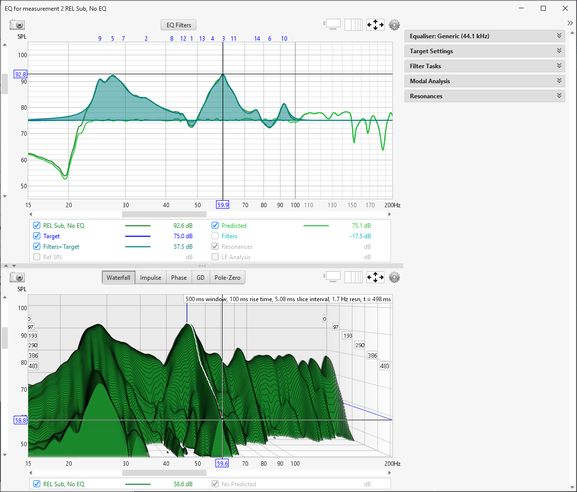
The EQ Window is used to determine what EQ filters to apply to a response and to see the effect those filters would have on both the frequency and time domain behaviour. It always shows the response currently selected in the main REW window, which can be changed from the REW main window or by pressing ALT + a measurement number (e.g. Alt+3 selects the third measurement) or using ALT+UP/ALT+DOWN to move through the measurements.
The window has 3 main areas: a "Filter Adjust" graph of frequency responses; a second graph area showing the impulse response, waterfall, phase, group delay and pole-zero graphs for the measurement and the predicted results of EQ; and a panel on the right with various settings related to the EQ functions and modal analysis. The right hand panel can be hidden/shown using the chevron button at the top of the scroll bar.

The Filter Adjust plot shows the measured and predicted (equalised) response for the current measurement along with the target response and the response of the equaliser filters with and without the target. This plot, in common with all plots that have a frequency axis, also optionally shows where any filters have been defined, displaying the filter's number along the top margin of the plot at the position corresponding to its centre frequency.
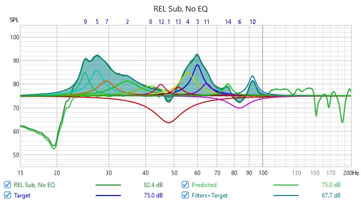
The frequency response of the measurement is labelled with the measurement name.
The Predicted response shows the predicted effect of the measurement's
filters. The Target trace shows the target frequency response for the
measurement, including any desired House Curve response shape. If a House Curve has been loaded the
![]() symbol will
be displayed by the trace value. The Target response includes the Bass Management
curve appropriate to the speaker type selected for the measurement in the
Target Settings. The Filters trace shows the combined
frequency response of the filters for this measurement, along with the individual
filter responses if this has been selected (see Filter Adjust Controls below). The Filters+Target
trace shows the frequency response of the filters overlaid on the Target
response. Selecting the filter responses to be drawn inverted and adjusting
the filters so that this curve matches the measured response will result in
the predicted response matching the target.
symbol will
be displayed by the trace value. The Target response includes the Bass Management
curve appropriate to the speaker type selected for the measurement in the
Target Settings. The Filters trace shows the combined
frequency response of the filters for this measurement, along with the individual
filter responses if this has been selected (see Filter Adjust Controls below). The Filters+Target
trace shows the frequency response of the filters overlaid on the Target
response. Selecting the filter responses to be drawn inverted and adjusting
the filters so that this curve matches the measured response will result in
the predicted response matching the target.
The control panel for the Filter Adjust graph has these controls:
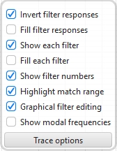
When Invert filter responses is selected the responses of the filters are drawn inverted. This is useful for graphically matching the shape of a filter to the shape of the peak it is being used to correct, when the shapes match the overall response in that region will be flat.
Fill filter responses fills the overall filter response. Show each filter draws the individual filter response shapes separately in different colours. Fill each filter fills the individual responses.
Show filter numbers controls whether the numbers of each filter are shown along the top of the graph.
The frequency span selected for target match is highlighted if Highlight match range is selected.
If Graphical filter edit is selected the gain or frequency of filters can be adjusted by clicking and dragging on the circular handles at each filter's centre frequency. The colour of the handles matches the colour of the filter in the EQ filters panel. Q can be adjusted by placing the mouse over the circular handle and using the mouse wheel. For fine Q adjustment hold the Alt key while moving the mouse wheel. Note that if Graphical edit is enabled it is not possible to zoom the graph with the mouse wheel, but zooming the X axis (mousewheel plus shift key) remains available when the mouse is not over a filter handle. The response of the filter is highlighted when the mouse is over the filter's handle.
Show modal frequencies controls whether the positions of the modes corresponding to the room dimensions entered in the Modal Analysis panel are shown along the bottom of the graph.
The Trace options button brings up a dialog to change the colours or line types of the graph traces, or hide some of them.
The EQ Filters panel is displayed by clicking
the button at the top of the EQ window.

The Waterfall plot shows a waterfall for the measurement and for the predicted result of applying the current filters to the measurement. The Predicted waterfall can be configured to update automatically as filters are adjusted (see Waterfall Controls below).
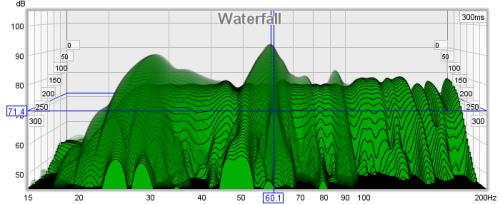
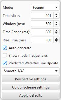
Mode would usually be Fourier to examine the time domain behaviour, but a Burst decay mode allows the plot to be generated with a period-based axis, the waterfall graph help has more on that.
The Predicted plot can be overlaid on the current measurement. The overlay is generated slice-by-slice, plotting a slice of the current measurement's waterfall, then a slice of the overlay, then the next slice of the current measurement and so on.
If Predicted Waterfall Live Update is selected the waterfall will be regenerated as filters are adjusted - it may take a few seconds for the update to appear, depending on the speed of the computer and the frequency span of the measurement. Note that the waterfall colour scheme is forced to "none" when using live updates as the colour scheme options slow down redraw.
The Total Slices control determines how many slices are used to produce the waterfall. Fewer slices mean faster processing, but make it less easy to see how the response is varying over time.
The width of the impulse response section that is used to generate the waterfall is set by the Window control (this control sets the Right Hand window width). The corresponding frequency resolution is shown to the right of the window setting. Longer window settings provide better frequency resolution.
The Time Range control determines how far the impulse response window is moved from its start position to generate the waterfall.
The Rise Time control sets the width of the Left Hand window. Shorter settings give greater time resolution but make the frequency variation less easy to see. The default setting, 100 ms, is aimed at revealing room resonances. When examining drive unit or cabinet resonances with full range measurements a much shorter rise time would be used, 1.0 ms or lower, with time spans and window settings of around 10 ms. CSD mode is often more useful for such measurements as the later part of the impulse response can be noisy, obscuring the behaviour in the later slices.
The Smoothing applied to the waterfall slices can be increased from 1/48th octave (the minimum, and recommended) to as high as 1/3rd octave.
The Perspective settings control the appearance of the plot including a Transparency setting which can be applied to the main plot, the Predicted overlay, or both. When transparency is set to 0% both plots are solid. The transparency mode can be switched between main/overlay/both to ease comparison between the plots.
The control settings are remembered for the next time REW runs. The Apply Default Settings button restores the controls to their default values.
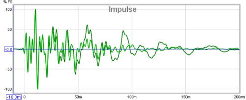
The Impulse plot shows the impulse response of the measurement and of the predicted result of applying the current filters to the measurement.
The Phase plot shows the phase response of the measurement and of the predicted result of applying the current filters to the measurement.
The Group Delay plot shows the group delay of the measurement and of the predicted result of applying the current filters to the measurement.
The area to the right of the graphs contains a group of collapsible panels containing settings that affect the EQ functions.
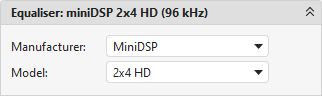
The Equaliser panel is used to select the type of equaliser that will be applied to the current measurement. Changing the equaliser type updates the filter panel, applying the settings appropriate to the selected equaliser. Filters already defined are retained where possible, but parameter values will be adjusted if necessary to comply with the ranges and resolutions of the chosen equaliser. The currently selected equaliser is shown in the panel title and in the EQ Filters panel. Details of the various equaliser types can be found here.
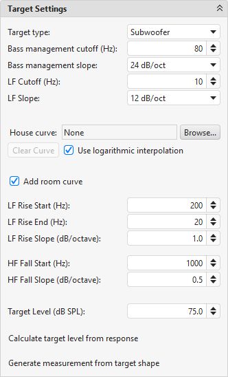
The Target Settings panel is used to tell REW what you expect or want the response to look like, so it knows what to aim for when applying EQ. The first selection (Target Type) should reflect the kind of speaker the measurement is from. If it's a Full Range ("Large") speaker the target is flat with a configurable low end roll off frequency (LF Cutoff) and slope (LF Slope). Setting the LF Cutoff to zero results in a target response that remains flat to 0Hz.
If it's a Bass Limited ("Small") speaker the target includes the effect of the bass management filter, the Bass management slope setting lets you tell REW how steep the bass management filter is and Bass management cutoff is the frequency it is set to, typically 80Hz in Home Theatre systems.
The Subwoofer target is similar, except the high frequencies are rolled off and there is a configurable low end roll off frequency and slope. For a 'Full Range' speaker the LF cutoff might be 40 Hz, for a sub it might be 20 - 30 Hz. You can usually see from the measurement where it is rolling off and adjust these settings for the target until it matches.
The bass management slope would typically be 24dB/octave for a subwoofer and 12dB/octave for a bass limited speaker, however the 12dB/octave figure for a speaker is used because the speaker itself is expected to have around a 12dB/octave acoustic roll-off, hence the overall effect of the filter and the speaker's roll-off is around 24dB/octave - the 24dB setting may be a better match to the measured response in those cases.
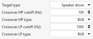
There is also a Speaker driver target type to use with measurements of individual drive units. Low pass and high pass crossover filters of up to 8th order can be configured to form the target.
A house curve file can be loaded which has a set of data that defines an offset
curve that is added to the target type shape and any room curve (see below for room
curve settings). The file containing the
house curve data is plain text consisting of pairs of frequency and offset
values separated by spaces, tabs or commas. Interpolation is used
between the pairs of values, either linear (default) or logarithmic,
according to the state of the Use logarithmic interpolation
check box. Logarithmic interpolation draws lines between data points which are
straight if the frequency axis is logarithmic. The first and last values in the file are used for all
frequencies below and above the range of the data respectively.
The house curve would typically be used to define a boost for the subwoofer range, such as that defined by the data points below. These points give a boost that is 6dB at 20Hz, dropping to 0dB at 80Hz and above. The boost remains flat at 6dB below 20Hz. A more elaborate curve might include a roll-off at high frequencies (if full range equalisation were being applied).
        House Curve data

        20 6.0
        80 0.0
When a house curve has been loaded the ![]() symbol is displayed next to the Target trace value in the Filter Adjust graph.
symbol is displayed next to the Target trace value in the Filter Adjust graph.
An Add room curve option is an alternative to specifying a house curve file that allows the target to to include typical room effects at the listening position and, if desired, a boost at low frequencies. HF Fall is used to reflect the downward tilt at high frequencies which is normal for most listening position speaker measurements, the result of the room's absorption and the speaker's power response. LF Rise allows that tile to be extended to low frequencies, to target a higher bass level which may be subjectively preferred. The target curve will rise below the LF Rise start frequency at the slope selected until reaching the LF Rise end frequency. Similarly, the target curve will fall above the HF Fall start frequency at the slope selected. The room curve effect can be turned on and off using the Add room curve box.
The Target Level control lets you move the whole target response up or down until it sits in the right place relative to your measurement. When the target is right the bits that go above it are the peaks you want to tame and it usually runs more or less through the middle of the measurement. Calculate target level from response automatically adjusts the level of the target response to provide a good match to the measurement over a suitable frequency range for the target type, but don't be afraid to manually adjust the level to suit.
Generate measurement from target shape creates a new measurement whose response matches the currently configured target. That measurement may be used on the RTA or the ALL SPL graphs to act as a reference.
The default target type, bass management slope, cutoff, LF rise and HF fall to use for new measurements are specified in the Equaliser Preferences.
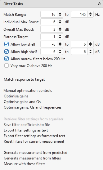
The Filter Tasks panel is used to control REW's automatic filter adjustment feature. REW can automatically assign and adjust filter settings to match the Predicted response to the target response.
The Match Range defines the frequency span over which REW attempts to match the target response, and within which filters will be assigned. REW can apply filters anywhere across the band, but it is usually best to limit filters to low frequencies (less than 200 Hz or so) unless you are compensating for some general characteristic in the speakers (an example might be a dip in the mid range or a bit too much HF) - that is using EQ as a fancy tone control.
Individual Max Boost sets the maximum boost that REW will allow for any individual filter. This can be set to zero to prevent REW assigning any boost filters.
Overall Max Boost sets the maximum boost that REW will allow for the combined effect of all the filters. This can be set to zero to prevent REW allowing any overall boost, but individual filters may still have boost. If the filter set has any overall boost the headroom this requires will be shown on the EQ filters panel.
In addition to the gain limits, boost filters are subject to Q limits to avoid inadvertently creating artificial resonances. The Q of boost filters is not allowed to exceed a value which would cause the filter's 60dB decay time to exceed approximately 500 ms (the actual Q limit value depends on the filter's gain).
The Flatness Target controls how tightly REW tries to match the Predicted response to the Target Response. The lower the Flatness Target, the more filters will be required.
Allow low shelf and Allow high shelf let REW use shelf filters at the beginning and/or end of the range to better match the response to the target. Shelf filters will only be used if the equaliser supports them and the response remains above or below the target for a span of at least half an octave at the beginning or end of the match range. The allowable gain range for the shelf filters is set to the right of the check boxes.
Allow narrow filters below 200 Hz determines whether target match uses filters narrow enough to counter modal resonances at low frequencies. This should be selected when applying EQ to a room measurement, but is best not selected when applying EQ to a device response (headphone EQ, for example). When this option is not selected the highest Q used will be 5.0.
If Allow narrow filters below 200 Hz is selected the Vary max Q above 200 Hz option tells REW to adjust the maximum Q from 10.0 at 200 Hz to 3.0 at or above 10 kHz. If this is not selected the max Q above 200 Hz will be 5.0.
Match Response to Target starts REW's automated filter assignment and adjustment process. REW assigns filters to match the Predicted response to the Target Response, beginning with the area within the Match Range where the measurement is furthest from the target. After assigning filters, REW adjusts the settings of the filters to get the closest match. It is best to apply the 'variable' smoothing to the response before running the target match.
For best results it is essential to first ensure the shape of the target response is correctly selected to suit the type of speaker whose response is to be equalised and set the Target Level so that REW does not end up applying filters to try and correct a level difference - equalisers are not volume controls!
Note that by default REW will not apply filters below the frequency at which the measurement first exceeds the target or above the frequency at which the measurement last drops below the target to prevent trying to boost a response beyond its natural roll-offs, if you wish to lift the low or high end response this can be done with manually applied filters but beware of exceeding the excursion limits or headroom of the woofer or power handling limits of the tweeter.
The Filter Tasks panel also includes a set of controls to optimise the settings of the current filters. Note that only filters that lie within the Match Range will be adjusted. Optimise gains will adjust the gains of all 'Automatic' PK and modal filters to best match the target response. Optimise gains and Qs will adjust the gains and Qs of all 'Automatic' PK filters and the gains of all 'Automatic' modal filters. Optimise gains, Qs and frequencies will adjust the gains, Qs and centre frequencies of all 'Automatic' PK filters and the gains of all 'Automatic' modal filters - it is equivalent to Match response to target without the automatic assignment of filters. Centre frequencies will be adjusted to within 10% of their initial setting and will remain within the match range.
If REW can read from the equaliser Retrieve filter settings from equaliser will be enabled, selecting it will read the settings either directly from the equaliser or from a file exported by the equaliser, depending on the equaliser type. Send filter settings to equaliser will transfer the current filter settings to the equaliser if the equaliser offers that capability. Save filter coefficients to file writes the biquad coefficients for the current filters at the selected sample rate in a form the equaliser can import. Export filter settings as text and Export filter settings as formatted text generate text files with the filter types and settings. Reset filters for current measurement will clear all the filters.
Generate measurement from predicted creates a new measurement whose response matches the predicted effect of any EQ filters. It has the same name as the current measurement prefixed by "EQ".
Generate measurement from filters creates a new measurement whose response matches the current EQ filters. It has the same name as the current measurement prefixed by "Filters". If there are no active filters the result is a perfect impulse.
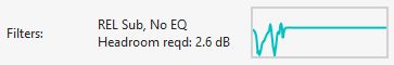
Measure with these filters will open the Measure dialog to make a new measurement with the current filter settings applied to the sweep. It provides a way to test the effect of filter settings on measurements without having an equaliser or when the equaliser is bypassed (for example, Windows software equalisers are usually bypassed when using WASAPI exclusive or ASIO drivers). The Measure dialog will show a small image of the filter response and any headroom requirement the filter set has. if the filter set has overall gain that needs to be taken into account to avoid clipping the output.
REW can analyse the low frequency part of the measured response to search for modal resonances. The search is controlled by the settings in the Modal analysis panel. To determine the modal characteristics a parametric analysis of a segment of the impulse response is carried out to identify the frequencies, amplitudes and rates of decay of the resonant features that make it up. Such an analysis is not constrained by the frequency resolution limits of an FFT, allowing precise values for each mode's parameters to be determined. However, the accuracy of the results depends on the signal-to-noise ratio of the measurement. The better the measurement, the better the results. To get the highest measurement quality for modal analysis set the sweep end frequency to match the highest frequency of interest and use a long sweep.
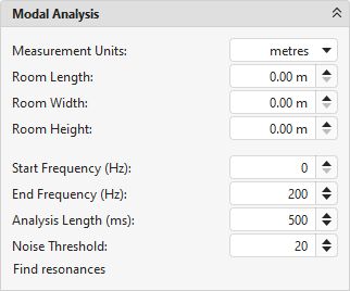
The modal analysis panel includes selections for the room dimensions. These are used to determine the room's theoretical modal frequencies up to 200 Hz, which may be plotted on the SPL & Phase, Group Delay, Spectral Decay, Waterfall and Spectrogram graphs. If any dimension is set to zero the corresponding modal frequencies will not be plotted, if all the dimensions are zero no modal frequencies will be plotted. The colours used for the modal frequencies are the same as those used in the Room Simulator.
The panel controls select the range to search for resonances (which will be restricted to the range of the measurement if smaller), the duration of the impulse response to analyse and a threshold for filtering out spurious resonances due to noise in the measurement. Best results are obtained by keeping the frequency span to around 100 - 200 Hz. The Analysis Length, 500 ms by default, may be reduced if the measurement is noisy or increased if the measurement has particularly low noise (noise floor of the impulse more than 60 dB below the peak).
Small alterations of the analysis length, 10-20 ms or so, can help establish whether the modal resonances identified are accurate - modes with consistent frequency, amplitude and decay time at differing analysis lengths indicate reliable data. When Find Resonances is clicked the analysis begins, it usually completes after a few seconds. The results are shown in the Resonances panel.
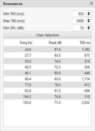
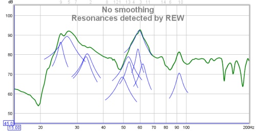
The Resonances panel includes controls to filter the results list according to the T60 decay times of the resonances and their amplitude. The list of resonances may be sorted by frequency, SPL ("Peak dB") or T60 decay time by clicking on the column headers in the table. Clicking on a resonance in the table will show a plot of its shape on the Filter Adjust graph, multiple resonances can be selected by clicking and dragging or using Ctrl+click or Shift+click. Clear Selection clears any selections made.
Filters which accurately counter specific resonances can be generated by selecting the "Modal" filter type and setting the Target T60 value to the T60 time determined by REW. Modal filters are normal parametric EQ filters whose Q or bandwidth is adjusted by REW as their gain is changed to ensure they target the specified T60 value as closely as the equaliser settings resolution permits.
REW provides a Pole-Zero plot as an alternative way of viewing the results of the modal analysis. This may be an entirely unfamiliar way of viewing a response to many, but it does have some virtues when looking at resonances and filters. However, little would be lost by ignoring this section.
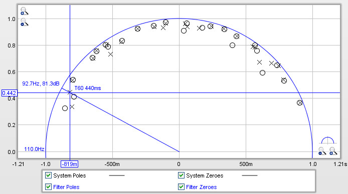
The pole-zero plot is a graph of complex numbers with the real part along the horizontal axis and the imaginary part along the vertical axis. There is a circle on the plot with a radius of one unit (referred to as the "unit circle") which corresponds in a way to the frequency axis of a frequency response. The plot shows results up to a frequency a little above the end of the modal analysis search, the upper frequency span of the plot is shown just to the left of the unit circle, near the point (-1, 0). As we move around the upper half of the unit circle the frequency increases from zero at the right side to the upper limit of the plot at the left. The lower half of the circle corresponds to negative frequencies, but for the signals we are looking at the bottom half is always a mirror image of the top half and can be ignored.
The plot shows poles, represented by crosses, and zeroes, represented by circles. Poles are places where the response becomes infinite, zeroes places where it becomes zero. The closer a pole gets to the unit circle, the more it pulls the frequency response upwards. Conversely, zeroes pull the response towards zero. Poles and zeroes at the same location cancel each other out completely, poles and zeroes close to one another partially counter each other's effects. If the plot has many pole/zero pairs that overlap they can be reduced by increasing the Noise Threshold setting. Poles outside the unit circle would correspond to an unstable system, none should appear there. Zeroes outside the circle would mean the response is not minimum phase, but the analysis may not start at the zero time of the impulse so this plot is not necessarily a good indicator of whether a response is minimum phase, for the correct method of determining that (using the excess group delay plot) refer to the Minimum Phase help topic.
Each modal resonance has a corresponding pole (actually a pair, the second is a mirror image below the axis). The frequency of the pole can be seen by drawing a line from the (0,0) point out through the pole to the point it reaches the unit circle, in the plot above the pole is at approximately 92.7Hz. REW shows the frequency value, and the SPL level at that frequency (81.3dB above). The closer a pole gets to the unit circle, the longer its T60 decay time. REW shows the T60 time corresponding to the cursor position, in the example above it is 440ms. If a resonance is selected in the Resonances panel its pole will be highlighted on the plot. The plot can be zoomed in on to get a closer view, clicking the button just above the x axis zoom buttons will reset the axis ranges to show the upper half of the unit circle.
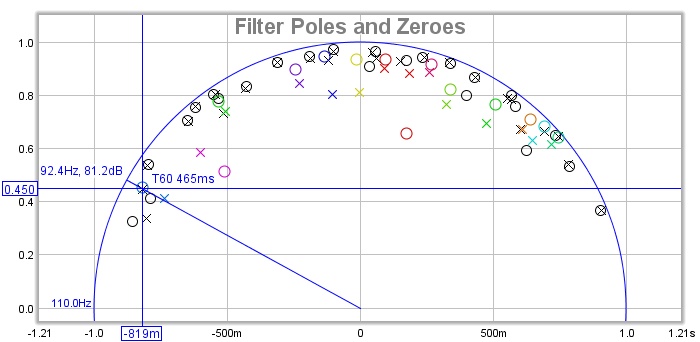
Filters also have poles and zeroes, a parametric EQ filter has a pair of poles and a pair of zeroes (one pole and one zero above the axis, the other below). The locations of the filter's poles and zeroes vary as the filter's settings (frequency, Q/bandwidth and gain) are adjusted. If the settings of a filter are adjusted so that its zero is directly over the pole of a resonance, it completely counters the effect of that resonance in the time and frequency domains. Seeing how filter zero locations compare to response pole locations is where the pole-zero plot can be useful. In the case of the "Modal" filter type REW makes the adjustments that keep the filter's zero at a distance from the unit circle that matches the filter's target T60 time.
Filter poles and zeroes are shown in colour on the plot, corresponding to the colour used for that filter on the filters panel and the Filter Adjust plot. An example of a set of filters is shown below. Filters that cut (negative gain) have their zeroes closer to the unit circle than their poles, filters that boost have their poles closer to the unit circle than their zeroes.
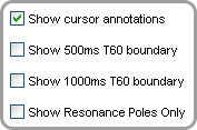
Show cursor annotations controls whether REW draws a line from the origin through the cursor position to the unit circle and labels the frequency, response SPL and T60 values. If Show 500ms T60 boundary or Show 1000ms T60 boundary are selected REW will draw circles on the plot corresponding to those T60 times, any pole outside those circles has a T60 time greater than the circle value. If Show Resonance Poles Only is selected the pole-zero plot will only show the poles for the resonances displayed in the Resonances panel, otherwise it shows all poles found during the analysis.