The Distortion graph shows the measurement's fundamental (the linear part of its response), its harmonic distortion components up to the ninth harmonic, Total Harmonic Distortion (THD) and the level of the noise floor, which is captured before the measurement starts.
The plots are derived either from analysis of the impulse response or from stepped sine measurements. Impulse responses measured using logarithmic sweeps separate distortion from the linear part of the system response. The distortion components appear at negative times, behind the main impulse. Analysing the frequency content of these components allows plots of distortion harmonics to be generated. The longer the sweep, the better the distortion components are separated from each other. Sweeps of 256k or shorter should start at 0 Hz to prevent an artificial rise in distortion at the lowest frequencies due to the reduced low frequency bandwidth of the resulting impulse response. When measuring a system with high distortion levels use a long sweep setting (e.g. 1M or higher), at shorter sweep lengths the harmonics may affect each other giving misleading results. A spot check can be made at frequencies of interest using the RTA and the signal generator. If discrepancies are observed consider making a stepped sine measurement instead. The noise floor of log sweep distortion measurements rises with frequency. For the lowest noise floor with sweep measurements use multiple sweeps, but note that requires the input and output to be on the same device for reliable results.
Although much, much slower than a log sweep the stepped sine measurement can measure low distortion levels much more accurately than a sweep, particularly at high frequencies and for higher harmonics. Stepped sine distortion measurements show distortion components up to the ninth harmonic, THD and the noise floor, in the same way as the sweep-derived results, but also include THD+N (total harmonic distortion plus noise and non-harmonic distortion) and N (noise and non-harmonic distortion) alone. Note that the noise floor plot shows the spectral content of the noise measured with no signal playing. The 'Noise' in the N and THD+N shows the summed level of all non-harmonic distortions and noise across the frequency span for each test frequency. It consequently sits much higher than the noise floor plot. For stepped level measurements the X axis can be dB SPL, dBFS, dBu, dBV, dBW, V or W showing either the generator or input level.
The harmonic plots can only be generated for frequencies within the bandwidth of the measurement. For example, if a measurement is made to 20 kHz, the second harmonic plot can only be generated to 10 kHz, as the 2nd harmonic of 10k Hz is 20 kHz. Similarly the third harmonic plot can only be generated to 6.67 kHz (20/3). The upper limit for distortion plots is 95% of the Nyquist frequency (which is half the sample rate). For example, at 44.1 kHz sampling the upper limit is 0.95*44.1/2 = 20.95 kHz.
The lower frequency limit for distortion plots is 10 Hz or the measurement start frequency, whichever is higher. 10 Hz is the lower limit of the logarithmic part of the measurement sweep. Start frequencies lower than that use an initial linear swept portion (to avoid spending an excessive proportion of the sweep duration time at very low frequencies) which means that region cannot be used to generate distortion data. Note that sweeps with start frequencies of 20 Hz or higher may show rising distortion at low frequencies as a result of the time domain ringing inherent in band limited impulse responses overlapping the distortion harmonics. To avoid that use start frequencies below 20 Hz where possible and longer sweeps.
Total Harmonic Distortion is generated from the available harmonics. There is a control to select the highest harmonic to use in the THD calculation, the trace name in the graph legend shows which harmonics are included. At higher frequencies the THD plot will incorporate fewer harmonics, according to which are available.
If the Analysis Preference Apply cal files to distortion is selected the results will include corrections for the cal file responses (as is the case for the RTA distortion figures). Applying the cal files provides more accurate results in regions where the fundamental or harmonics are affected by interface roll-offs but boosts the noise floor in those regions. This should be borne in mind when viewing the results. If large cal file corrections are required make sure the Analysis Preference Limit cal data boost to 20 dB is not selected. Note that any subsequent changes to the cal files will NOT update the distortion results, they are generated from the cal files that were in use at the time the measurement was made.
When measurements with distortion data are averaged their distortion data is also averaged, providing the measurements were made over the same frequency range and at the same resolution.
The fundamental and harmonic plots derived from sweep measurements are smoothed to 1/24 octave. This cannot be adjusted. The distortion data can be exported to a text file using File → Export → Distortion data as text.
The control panel for the graph has these controls:
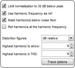
By default the plot shows the absolute levels of the fundamental and the harmonics. The Y axis can be set to show dB SPL, dBFS, dBu, dBV, dBW, volts, watts, dBr or percent. Values for dBW and watts are derived from the measured voltages using the reference impedance value in the RTA Appearance settings. If the Y axis is set to percent or dBr the harmonics are divided by the fundamental to show their relative level and the fundamental appears as a flat line at 0 dBr or 100%. The legend value for the fundamental will continue to show its absolute level, the readings for the harmonics and THD will depend on the Distortion Figures setting. Normalising the plot will cause the distortion traces to rise at high frequencies if the response of the system being measured rolls off (as is usually the case). This is exaggerated if Use harmonic frequency as ref is selected (see next section). The boosting due to low fundamental level can be controlled by selecting Limit norm. to 30 dB below peak, this sets a lower limit on the fundamental that is 30 dB below the peak level of the fundamental - for example, if the peak of the fundamental were 95 dB the minimum level used for normalising would be 65 dB.
The harmonic and THD plots in normalised mode use the level at the fundamental for each frequency as their reference by default - for example, the distortion figures for each harmonic at 1 kHz will depend on the level of the fundamental at 1 kHz. If Use harmonic frequency as ref is selected the reference will be the frequency of the harmonic - for example, at 1 kHz the 2nd harmonic figure will depend on the level of the fundamental at 2 kHz, the 3rd harmonic will depend on the level of the fundamental at 3 kHz and so on. This follows a recommendation made by Steve F. Temme in "How to graph distortion measurements" presented at the 94th AES convention in March 1993. If the response of the system being measured is flat this makes no difference to the results, but when the response is not flat (as for most acoustic measurements) it can remove the influence of the loudspeaker's fundamental response from the distortion figures. As an example, suppose the loudspeaker response was flat apart from a 6 dB peak at 2 kHz. 2 kHz is the 2nd harmonic of 1 kHz, so the 2nd harmonic level shown at 1 kHz will be increased by 6 dB due to the boost in the fundamental when using the excitation frequency as the reference. Similarly the 3rd harmonic level at 667 Hz (2/3 kHz) will be boosted by 6 dB. If the harmonic frequency were used as the reference the distortion figures would not show this boost. Using the harmonic frequency as the reference also provides a more meaningful view of distortion at frequencies below the LF roll-off of the system as otherwise the distortion levels are boosted as the level of the fundamental drops. Note that this option will not affect the traces when the plot is not normalised, but will still affect the values in the legend if the distortion figures are set to read in percent or in dB relative to the fundamental.
The Mask harmonics below noise floor control greys out harmonics that lie below the noise floor (at the frequency of the harmonic). The THD trace is also greyed out if all the harmonics that contribute to it are below the noise floor. In applying the masking for sweep measurements REW takes into account the (limited) ability of the sweep to discriminate harmonics that lie a below the noise floor at the harmonic frequency, which varies from 3 dB for the second harmonic to almost 10 dB for the ninth.
Plot harmonics at the harmonic frequency changes the way the harmonic orders for sweep measurement distortion are plotted - rather than plotting the distortion at the frequency of the fundamental it is plotted at the frequency of the harmonic, so (for example) the 2nd order harmonic distortion level for 1 kHz would be plotted at 2 kHz, where the distortion occurs. This makes it easier to correlate harmonic levels with the level of the fundamental at the harmonic frequency and also helps distinguish the effects of external noise, since noise affects all harmonics at the frequency at which it occurs. The THD trace is not affected by this control, it will continue to show the THD value corresponding to the harmonic levels at their fundamental frequency. However, when plotting harmonics at the harmonic frequency the level of the fundamental at the harmonic frequency (which in this graph mode is the cursor frequency) is used as the reference, so Use harmonic frequency as ref will be selected and the control for it disabled. If that was not previously selected the THD trace will update.
The Distortion figures control selects the units that are used for the harmonic distortion levels displayed on the graph legend. The choices are As Y axis, which shows the level using the selected Y axis unit; dB relative, which shows how many dB the harmonic is below the fundamental; and Percent, which shows the harmonic level as a percentage of the fundamental. The frequency at which the fundamental level is taken depends on the setting of Use harmonic frequency as ref (see above).
The Highest harmonic to show control allows the higher harmonics to be hidden if they are not of interest. For example, if Highest Harmonic to show were set to 3 only the second and third harmonic traces would appear on the graph and in the graph legend. The measured harmonics used to calculate THD are controlled by Highest harmonic in THD.
The Highest harmonic in THD control allows the higher harmonics to be excluded when calculating THD. This may be desired if they are in the noise floor and so adding noise to the THD calculation.
The Trace options button brings up a dialog that allows the colour and line type of the graph traces to be changed. If a change is made it will be used for all measurements shown on this graph. Traces can also be hidden, which will remove them from the graph and from the graph legend.
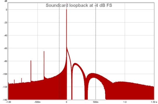
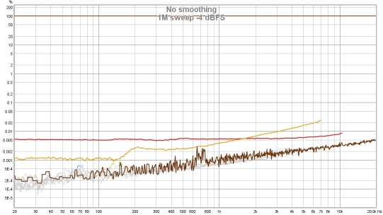
Here is a distortion plot generated from a loopback measurement of a soundcard, produced at a high sweep level (-4 dBFS, which resulted in 2 dB of headroom at the gain settings used). The readings in the legend are with the cursor at 1 kHz.
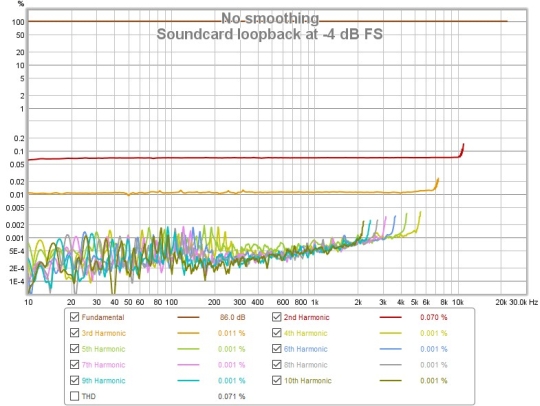
The THD trace has been omitted, as it overlays the 2nd harmonic trace (in red) which is the dominant component, 0.07%. The 3rd harmonic (in orange) is much lower at around 0.01%, whilst the higher harmonics are largely within the noise floor.
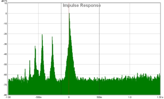
This is the impulse response for that measurement, the distortion peaks are to the left of the main peak. The first peak to the left is the 2nd harmonic, the next is the third harmonic and so on.
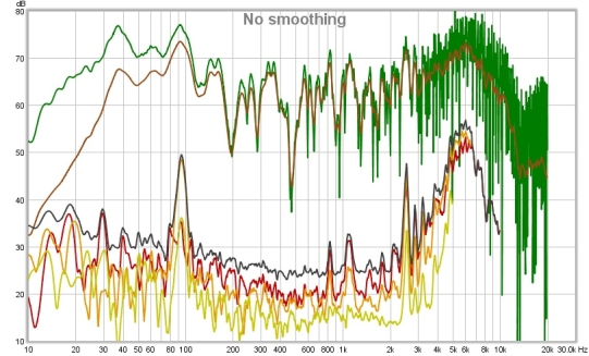
The next plot is from a room measurement. The 2nd (red), 3rd (orange) and 4th (yellow) harmonic traces are shown, along with the THD (black). Higher harmonics were within the noise floor. The measurement shows a sharp rise in 3rd harmonic distortion at 94 Hz, and a dramatic rise in all distortion components from about 2 kHz upwards. Further measurements at differing signal levels established that this distortion was being introduce by the SPL meter used for the measurement.
This is the impulse response for the in-room measurement, the distortion peaks are clearly visible to the left of the main peak.
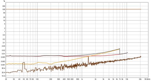
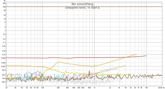
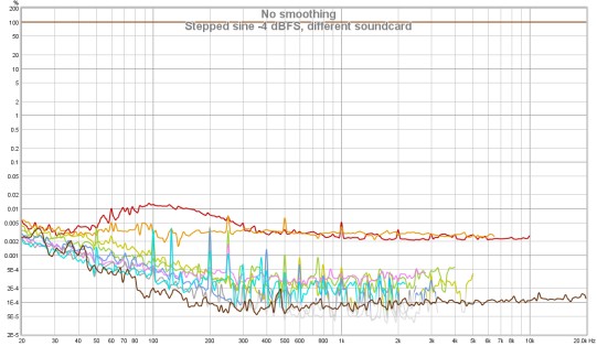
The plots below show a different soundcard loopback measurement at -4 dBFS measured with
stepped sine (64k FFT, 24 ppo) and with a 1M log sweep. Note the rise in the noise floor with
frequency when measuring with the sweep, all but the 2nd and 3rd harmonic lie below the noise
floor. In addition, the 3rd harmonic measures higher with the sweep than with stepped sine at
frequencies above 100 Hz or so. With the stepped sine measurement the contributions of the 4th,
5th and 7th harmonics are also visible above the noise floor (dark brown trace). Stepped sine
is a much more accurate method when measuring low distortion levels.
Further insight into the distortion behaviour can be obtained by looking at waterfall
or spectrogram views of the spectrum data captured at each test frequency. Note that these
can only be generated for stepped sine measurements that had the option to
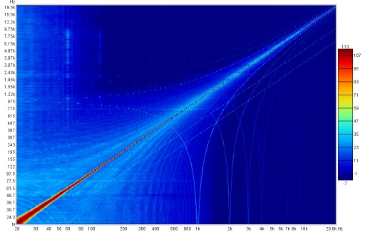
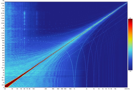
Capture spectrum data at each frequency selected. Here is a spectrogram of the stepped
sine measurement above.
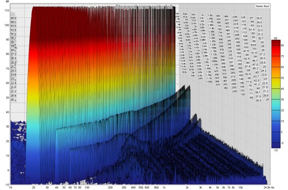
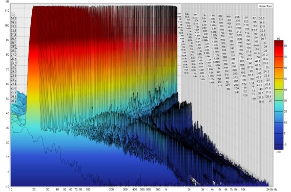
Here is its waterfall plot.
Here is a stepped sine measurement of another soundcard, superficially looking to have similar
performance to the one above.
However, its spectrogram makes clear that it has far worse behaviour with significant intermodulation
products with the 1 kHz harmonics of the USB frame rate.
Its waterfall plot is similarly revealing.
Speaker measurements, particularly those made in-room rather than with the benefit of an anechoic chamber, present additional challenges for interpretation. Distortion results for electronic components are typically shown as percentages, values relative to the fundamental. Plotting these percentages for speaker measurements can make the results challenging to interpret due to the often highly irregular frequency response of the speaker. Using the harmonic frequency as reference (see distortion controls above) helps somewhat, but is by no means a complete solution. My personal preference is to view the distortion results without normalisation, which helps make the effect of the response irregularities apparent and also emphasises the acoustic level of the distortion components, which can be helpful in deciding where they are likely to be audible and where not. When viewing the distortion graph as SPL levels the trace legend can still be configured to read out distortion percentages using the Distortion figures control.
Here is a measurement of a small desktop speaker (Adam Artist 3). The mic (UMIK-1) was
just 15 cm from the speaker, hence the relatively high SPL measured - the levels correspond
to about 85 dB at the listening position, about 70 cm from the speakers.
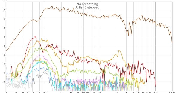
The hump of odd harmonics centred around 80 Hz or so looks to be mild clipping. Above 3 kHz,
where the speaker's ribbon tweeter comes into play, distortion levels drop below the noise floor
for the sweep though the stepped sine tracks them comfortably. As this is a near field measurement
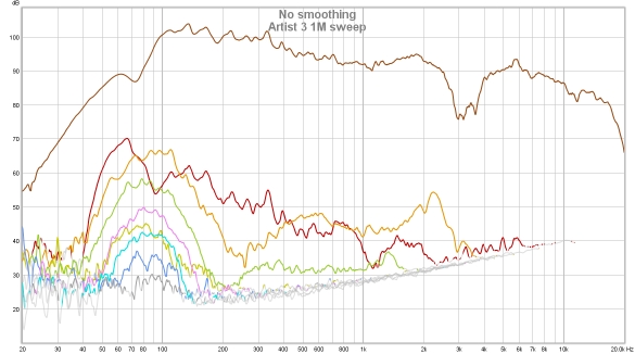
room effects are reduced, but the frequency response variation can still make a normalised view
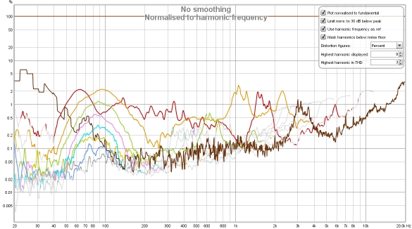
more difficult to fathom. Below is the response normalised, without using harmonic frequency as
ref. The noise floor (dark brown) is included to help illustrate the effect normalisation has on
boosting the noise floor where the response dips.
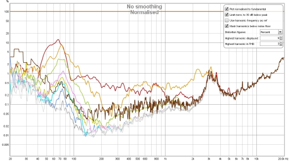
It is apparent that the peak in second harmonic distortion around 3 kHz is simply the noise floor being boosted and so can be ignored - though that would not be so easily identified without the noise floor trace to guide us. However, distortion at low frequencies is now shown much higher than it should be due to the low frequency roll off of the speaker's response meaning it is being normalised against a much lower level. That 10% 2nd harmonic might give cause for concern until it is recognised as an artefact of the normalisation.
The normalisation artefacts at low frequencies can be ameliorated by using the level of the
fundamental at the harmonic frequency as the normalisation reference. That gives us the plot below,
the low frequency behaviour is now more accurately portrayed. However, new peaks have appeared in
the 2nd and 3rd harmonics above 1kHz, consequences of the dip in the response centred around 3 kHz.
That dip is probably due to the crossover between mid/bass and tweeter integrating poorly at such a
near field measurement position. It is unlikely that the distortion peaks are real. The view without
normalisation is least susceptible to misinterpretation.