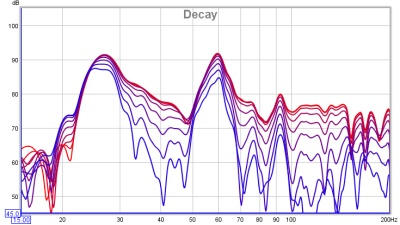
This graph shows spectral decay traces. The plot used logarithmically spaced data at 96 points per octave with 1/48th octave smoothing applied. The Spectral Decay plots are generated by shifting the impulse response window to the right by the slice interval to generate each succeeding slice. Two windows are used, a left side window to taper the data prior to the start of the region being analysed and a right side window that spans the selected window width. The default window type for the left side is Hann, for the right side it is Tukey 0.25, other types may be selected via the Spectral Decay entries in the Analysis Preferences. The initial reference point for the windows (end of left window/start of right window) is the peak of the impulse response.
The plot is generated automatically when the graph is selected, or may be
manually regenerated using the Generate button in the bottom left
corner of the graph area.
Right clicking on the graph brings up a menu of actions:
The Smoothing applied to the slices can be increased from 1/48th octave (the minimum, and recommended) to as high as 1/3rd octave.
Export data allows the SPL values for the time slices to be exported as text.
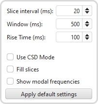
The time separation of the slices is controlled by the Slice Interval setting, the width of the impulse response section that is used to generate the slice is set by the Window control. The corresponding frequency resolution is shown to the right.
The Rise Time control sets the width of the Left Hand window. Shorter settings give greater time resolution but make the frequency variation less easy to see. The default setting, 100 ms, is aimed at revealing room resonances. When examining drive unit or cabinet resonances with full range measurements a much shorter rise time would be used, 1.0 ms or lower, with time spans and window settings of around 10 ms. CSD mode is often more useful for such measurements as the later part of the impulse response can be noisy, obscuring the behaviour in the later slices.
Use CSD Mode should be selected if the later slices of the decay are contaminated by noise in the measurement. It would commonly be used when examining drive unit or cabinet resonances. CSD mode anchors the right hand end of the window at a fixed point and only moves the left side. This does mean, however, that the frequency resolution reduces (and the lowest frequency that can be generated increases) as the slices progress, as each has a slightly shorter total window width than the previous slice.
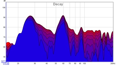
The traces for each slice can be drawn as conventional lines or as filled
areas, selected by the Fill slices check box. The alternative views
are shown below.
If Show modal frequencies is selected the theoretical modal frequencies for the room dimensions entered in the Modal Analysis section of the EQ Window are plotted at the bottom of the graph.
The control settings are remembered for the next time REW runs. The Apply Default Settings button restores the controls to their default values.