The SPL and Phase plot (or Impedance and Phase for an Impedance measurement) shows the frequency and phase responses of the measurement. The frequency response is labelled with the measurement name, the phase response uses a dotted trace and the right hand plot Y axis. The left hand Y axis can be set to show dB SPL, dBFS, dBr, dB V/V, dBu, dBV, dBW, volts/√(Hz), watts or, for impedance traces, ohms. The dBr and dB V/V values are effectively a transfer function view, showing either the relative input to output dBFS levels (dBr) or voltage levels (dB V/V). Values for dBW and watts are derived from the measured voltages using the reference impedance value in the RTA Appearance settings. The volts/√(Hz) axis option is only valid for RTA measurements.
For stepped level measurements the graph will show a plot of the input level versus the generator level, and a linearity plot showing the ratio of input level to generator level. There is an option in the graph controls to normalise the linearity trace so that it is at 0 dB at the end of the trace.
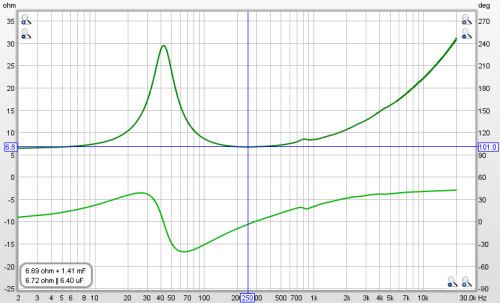
For impedance measurements the magnitude, phase and resistance (real part) of the impedance can be plotted, along with the Equivalent Peak Dissipation Resistance (EPDR). EPDR is used to evaluate how difficult a load a speaker's impedance presents by showing the resistance that would result in the same output device peak power dissipation as the speaker load at a given frequency, see E. Benjamin, "Audio Power Amplifiers for Loudspeaker Loads", JAES, Vol.42 No.9, September 1994.
when the mouse cursor is within the graph panel for an impedance measurement
the equivalent series resistance + inductance or resistance + capacitance
and parallel resistance||inductance or resistance||capacitance of the impedance
at the cursor position is shown at the bottom left corner
of the graph. This may be useful when making measurements of inductors or
capacitors to check their value, but the
Component Model provides a much more accurate equivalent circuit.
Note that to have valid phase information it is necessary to remove any time delays from the Impulse Response. A time delay causes a phase shift that increases with frequency - for example, a delay of just 1 ms results in a phase shift of 36 degrees at 100Hz but 3,600 degrees at 10kHz, because 1 ms is 1/10th of the 10 ms period of a 100Hz signal but is 10 times the 0.1 ms period of a 10kHz signal, and each period is 360 degrees. The time delay of a measurement can be adjusted by changing the zero position of the time axis using the Offset t=0 controls, or by using the Estimate IR delay control (Ctrl+Alt+E), both described below.
In addition to the measured phase, the plot can show minimum and excess phase plots that result from generating a minimum phase version of the response, described further below. The plot also shows any mic/meter or soundcard calibration data for the measurement. The calibration data can be changed or removed by selecting Change cal in the measurement panel right click menu.
If the Generate minimum phase action has been used to produce a minimum phase version of the response the minimum and excess phase traces are activated. The minimum phase trace shows the lowest phase shift a system with the same frequency response as the measurement could have, while the excess phase trace shows the difference between the measured and minimum phase. Note that it is best to make full range measurements if the minimum phase response is to be generated as a good result relies on measuring far beyond the bandwidth of the system being measured. Even then there are limits to the accuracy of minimum phase responses generated from sampled data, particularly at frequencies above about one quarter of the sample rate. There are options to improve the result, for details see Generating minimum phase below. For more about minimum and excess phase and group delay see Minimum Phase.
The Mic/Meter Cal trace shows the frequency response of the Mic calibration data for this measurement (the calibration file to use for new measurements is specified in the Cal files Preferences). If C Weighted SPL Meter was selected this curve will show the effect of C weighting (outside the range of the calibration data file, if there is one). The trace is not shown if there is no mic/meter calibration data. The trace is drawn relative to the middle of the graph.
The Soundcard Cal trace shows the measured frequency response of the soundcard relative to its level at 1kHz (if a calibration file has been loaded via the Soundcard Preferences). The trace is not shown if cal data has not been loaded. The trace is drawn relative to the middle of the graph. Fractional octave smoothing can be applied or removed via the Graph menu and its shortcut keys. The smoothing is applied to the SPL, phase and Group Delay traces. This is mainly used for full range measurements, as reflections can cause severe comb filtering which makes it difficult to see the underlying trend of the response. Smoothing should rarely be used for low frequency measurements as it obscures the true shape of the response. When smoothing has been applied an indicator appears in the trace legend.
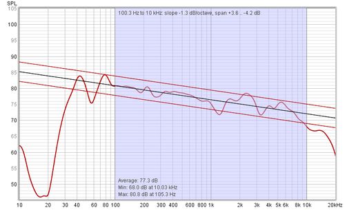
If a frequency range is selected by holding the shift key then pressing and dragging with the left mouse button a best-fit line for the selected range is displayed, with lines above and below it to show +3 dB and -3 dB. The slope of the line in dB/octave is shown (if the frequency axis is logarithmic) along with the span of the data relative to the best-fit line and the minimum, maximum and average of the range. The range can be adjusted after selection by dragging the start or end of the area, or the whole range can be moved.
Right clicking on the graph brings up a menu of actions:
The control panel for the SPL and Phase graph has these controls, there may be more or fewer controls depending on the measurement type.
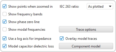
If Show points when zoomed in is selected the individual points that make up the SPL and phase responses are shown on the graph when the zoom level is high enough for them to be distinguished (which may only be over part of the plot)
If Show frequency bands is selected the audio frequency bands are shown in a stripe above the graph. The bands are:
Show phase zero line is selected a line is drawn at the zero phase position, this may not coincide with a grid line as the grid lines are linked to the left hand graph axis.
Show room panel is only shown for measurements generated from the Room simulator. If selected a plan view of the room configuration used to generate the simulated response is shown.
Show distortion panel is only applicable for measurements saved from the RTA with valid distortion data. If selected the distortion information is shown.
If Show modal frequencies is selected the theoretical modal frequencies for the room dimensions entered in the Modal Analysis section of the EQ Window (or in the Room simulator for responses generated from there) are plotted at the bottom of the graph.
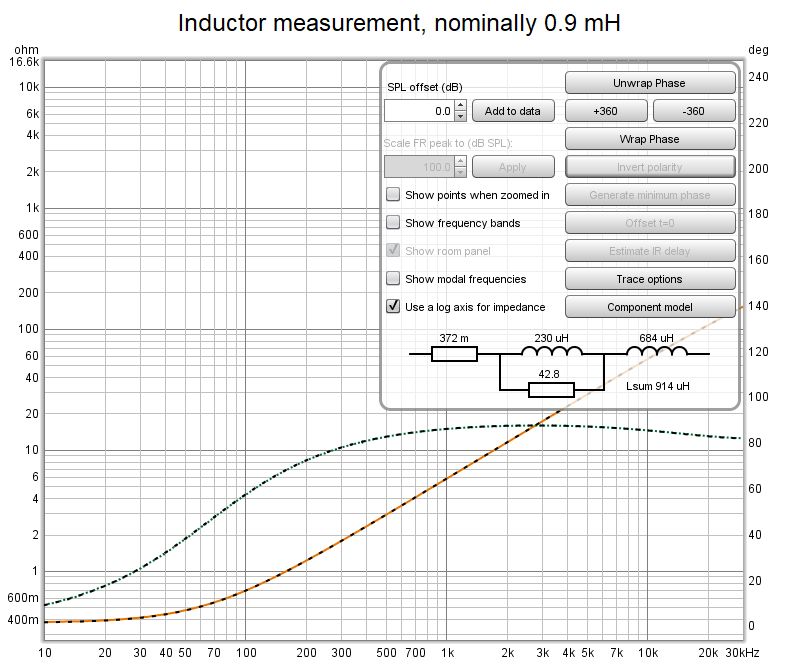
When impedance is being plotted the linear axis has a span from 0 to 1 kohm. If a larger impedance range is required the axis can be switched to logarithmic with a range up to 10 Mohm using the Use a log axis for impedance check box. If selected a log axis will be used wherever impedance is plotted.
The IEC 263 ratio control allows the graph to be locked to a specified dB/decade aspect ratio. The aspect ratio is maintained by adjusting the margins around the graph as required.
The Trace options button brings up a dialog that allows the colour and line type of the graph traces to be changed. If a change is made to a measurement trace it will be used for all measurements shown on this graph, overriding the measurement colour. Traces can also be hidden, which will remove them from the graph and from the graph legend.
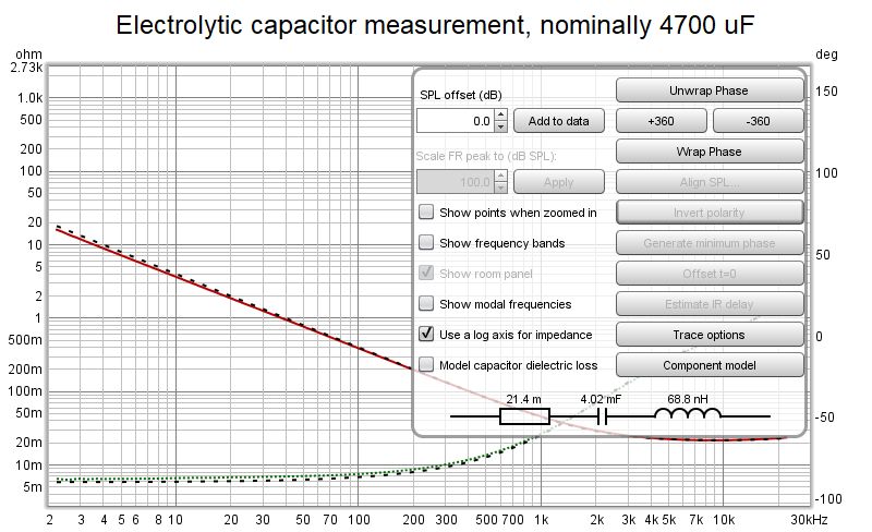
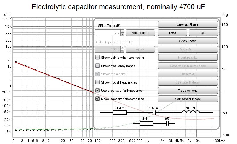
The Component model button is only shown for impedance measurements and only enabled for measurements of inductors or capacitors. REW identifies the measurement as being of a capacitor if the phase at 20 Hz (or the start of the measurement, if higher) is below -60 degrees, or an inductor if the phase at the end of the measurement is above 45 degrees. For those measurements pressing the button will carry out a curve fit over the range from 10 Hz to 20 kHz for inductors or 100 Hz to 20 kHz for capacitors (or the measurement range if smaller) to derive equivalent circuit component values. Measurements should span at least those ranges, preferably beyond them so that the model behaviour can be seen beyond the fit range. The equivalent circuit is shown below the button. The equivalent circuit impedance and phase are shown as dashed lines overlaying the measured traces. When measuring components make sure the component lead length is close to the length it will have in circuit, otherwise the measurement will include lead resistance and inductance which will not be present when the part is used.
For capacitors the equivalent circuit is a series combination of a resistor (the ESR), a capacitor and an inductor (likely to be very small at audio frequencies, not shown if less than 1 nH). The ESR value is likely to be over-estimated for very small capacitors (below 100 nF or so) as the impedance at the end of the model fit range (20 kHz) is still quite high, so it is limited to 1 ohm maximum in those cases. If the option to Model capacitor dielectric loss is selected an additional R and C may be included in parallel with the capacitor, to capture the effects of dielectric loss. The dielectric loss components are omitted if the loss capacitance is less than 0.1% of the main capacitance. The series R is omitted if it is less than 1 milliohm. Whilst accounting for the dielectric loss usually gives a more accurate fit to the impedance data the equivalent circuit becomes more complex and does not yield a single capacitor value to use. A combined Csum capacitance value is shown, but this may only be valid at low frequencies. The best option if a single figure is required is to use the impedance readout value shown at the bottom left of the graph when the cursor is at the frequency of interest. The images below show results without and with dielectric loss components.
For inductors the equivalent circuit is an LR2 model consisting of a series resistor, a series inductor and a resistor and inductor in parallel.
Generate minimum phase will produce a minimum phase version of the measurement. Using this control also generates a minimum phase impulse plot and, for measurements that already had an impulse response or phase data, minimum and excess phase and group delay plots. If the measurement did not have an impulse response but did have phase data an impulse response is generated using the original phase data. If the measurement only had SPL data the minimum phase impulse is set as the IR for the measurement, this allows an IR and phase to be produced for measurements which do not have them, such as imported text files.
If the system that was measured was inherently minimum phase (as most crossovers are, for example) the minimum phase response should be the same as removing any time delay from the measurement. Individual driver measurements are usually minimum phase, but multi-driver loudspeaker measurements are usually not. Room measurements are typically not minimum phase except in some regions, mainly at low frequencies. For more about minimum and excess phase and group delay see Minimum Phase.
There are limits to the accuracy of the minimum phase response that can be generated for sampled data systems which mean they may not reflect the true minimum phase response of the system being measured, particularly at frequencies above about one quarter of the sample rate. DAC reconstruction and ADC antialias filters are commonly not minimum phase and have very steep roll-offs, so results for systems whose bandwidth exceeds half the sample rate will be affected by them. REW's responses are generated by using the FFT, which means they will have zero phase at DC and half the sample rate. REW uses the real cepstrum to produce its minimum phase response.
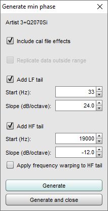
If Include cal file effects is selected the response used to generate the minimum phase will include any calibration files the measurement has. That means their influence will become part of the minimum phase impulse response. Note that measurement impulse responses themselves do not include cal file effects.
If the measurement does not cover the full frequency span from 0 to half the sample rate, or the device response drops into the noise floor at its extremes, there are options to define what data the minimum phase calculation should use outside the measurement range or the valid range of the measurement. The first option is to Replicate data outside range, which repeats the measurement start value for frequencies below the start frequency and the end value for frequencies above the end frequency. This may be useful for measurements that cover a limited frequency span, or have been imported from text files with a limited span.
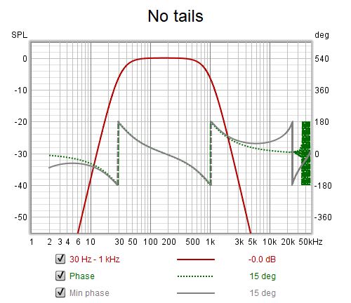
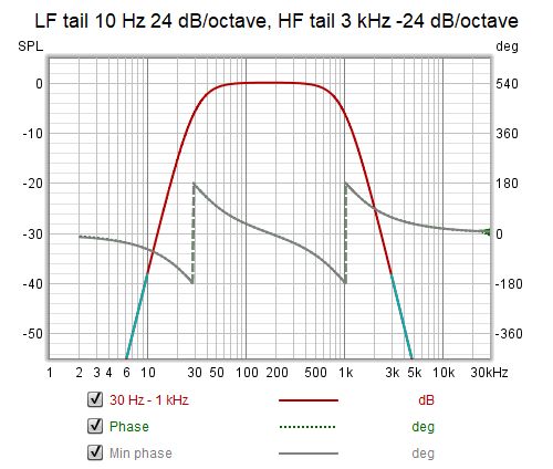
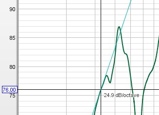
An alternative is to add 'tails' to the measurement at low frequencies, high frequencies or both. Some systems will have a known low frequency roll-off. For example, sealed box loudspeakers ultimately roll off at 12 dB/octave, while ported loudspeakers typically roll off at 24 dB/octave (in both cases below their respective resonant frequencies). The measured low frequency response can be replaced by a tail with a user-defined slope to facilitate the generation of an accurate low frequency minimum phase response. To help with this a slope overlay is shown at the cursor position, indicating the local slope of the response.
A tail may also be added at high frequencies, though the results may be less successful if the bandwidth of the system being measured is not far below the sample rate. If a high frequency tail is being added REW will oversample the response by a factor of 4 to reduce the influence of the sample rate. There is also an option to Apply frequency warping to HF tail which replicates the effect approaching half the sample rate typically has on the slopes of digitally-generated filters.
The images below show the effect of adding tails to a crossover response measurement. The tails are overlaid on the measurement in cyan. The result is very good, but this is an ideal case for the high frequency behaviour since the crossover was measured at 96 kHz and rolls off from 1 kHz, so the measurement bandwidth far, far exceeds the system bandwidth.