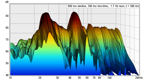
This graph shows a waterfall plot over the region from 10Hz to the end
of the measurement. It can be used to view the results of sweep measurements,
imported audio files or stepped sine measurements for
which the spectrum data has been captured at each measurement frequency. Measurement
and audio file plots can be generated in either Fourier or Burst Decay modes. A Fourier
plot is classical waterfall, produced by sliding a window along the impulse response or data
(a more detailed explanation is provided below). A Burst Decay plot
shows how tone burst decay along a decay axis of periods of the decay frequency, making it
easier to compare the Q of resonances. The plot is generated automatically when the graph
is selected, or may be manually regenerated using the Generate button in the bottom
left corner of the graph area.
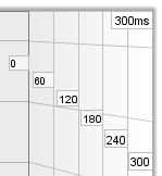
The labels at the sides of the plot show the decay axis values, in either time or,
for Burst Decay, periods.
To understand what the Fourier waterfall plot shows and how its appearance is affected by the various waterfall controls it is helpful to first understand how it is generated.
Each slice of the waterfall plot shows the frequency content of a windowed
part of the measurement's impulse response. 'Windowed' means we take the impulse
response and multiply each sample in it by the value of a window, which is made up
of a left side and a right side whose shapes we can choose (the window types are
selected via the Spectral Decay entries in the Analysis Preferences).
Here is an example of an impulse response showing the original impulse, the window
shape (in blue) and the windowed response.
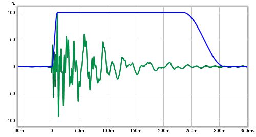
Here is a zoomed in view of the early part, where the effect the windowing has
on the windowed (lighter green) trace can be seen.

After the frequency content of the first windowed part of the impulse response has been obtained it is plotted as the first slice of the waterfall. The window is then moved along the response and the process is repeated for the next slice. The amount the window moves is determined by the time span of the waterfall and the number of slices that are to be plotted, so that the data for the last slice is from a section of the impulse response that is later than the first slice by the time range - for example, if the time range was 300 ms and there were 51 slices there would need to be 50 shifts of the window (the first slice has no shift) so each slice would be from data obtained after moving the window 6 ms along the impulse (300/50).
The window has a left hand side and a right hand side. In the plots above, the left hand window is a Hann type that ends at the peak of the impulse. The right hand side is a Tukey 0.25 (which means that for 75% of its width it is flat, then the remaining 25% is a Hann window). The overall width of the window (left side plus right side) determines the frequency resolution of each slice of the waterfall. The shape of the window, and particularly the shape and width of the left hand side, affects the way features of the response are smeared out in time.
To understand this, imagine a rectangular window and a perfect impulse, that has one sample at 100% and all other samples zero. As long as that single 100% sample is within the span of the window the frequency response will be a flat line. As soon as the left edge of the window goes past the 100% sample that slice and all slices after it will have no data in them (all the samples will be zero) so the waterfall would disappear off the bottom of the plot. Here is an example of such a waterfall plotted with a 100 ms left hand rectangular window.
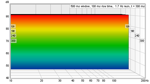
That waterfall is, in the time domain, a faithful representation of how that perfect impulse response looks - and in general for any response a rectangular window gives the best time resolution, but that comes at a price. The price is in the frequency domain behaviour, i.e. the shape of the frequency response in slices of the waterfall. In real impulse responses, that are spread out over time, using a rectangular window creates a sharp step at the left hand edge of the windowed data. That sharp step causes ripples in the frequency response, obscuring the actual frequency content. The waterfall also has an initial period, equal to the width of the left hand window, where the slices are almost identical, creating a flat portion. Here is an example of a measurement with a 100 ms rectangular left hand window, despite its appearance it is the same measurement as shown at the top of this help page, only the shape of the left hand window has been changed.
To avoid the damaging effects of that sharp step in the windowed response, a tapered window is used to smoothly attenuate the samples, but now a feature that does actually have a rapid change in the impulse response will linger on in the waterfall, because it will not entirely disappear until the whole left hand window has gone past it. Here are the perfect impulse and the real measurement again, this time with a 100 ms Hann left hand window.
REW's sweep measurement waterfalls are aimed at examining room resonances. To help make those resonances easy to see in the response, a wide left hand window is used. The left hand window width is specified independently, using a setting labelled Rise Time. Changing the Window setting only alters the Right Hand window, which means that the Window setting now controls only the frequency resolution of the waterfall - longer settings give higher resolution - without altering the waterfall's time domain behaviour. There are also controls to select how many slices the waterfall should have and to select the smoothing to apply to each slice.
In addition to the standard waterfall mode, which slides the window along the impulse response, there is a CSD (Cumulative Spectral Decay) mode, which anchors the right hand end of the window at a fixed point and only moves the left side, which may be useful when examining cabinet or tweeter resonances over very short time spans if the IR data descends into the noise floor soon after the region being examined. Using CSD mode in those cases prevents the later slices from including increasing amounts of noise floor. This does mean, however, that the frequency resolution reduces (and the lowest frequency that can be generated increases) as the slices progress, as each has a slightly shorter total window width than the previous slice. Note also that it does not make sense to have a time range greater than the window width in CSD mode as the window, with its fixed right hand edge, reaches zero width after stepping along by a time interval equal to the window width and there will be no data for subsequent slices. In CSD mode window width should be greater than the time range. CSD mode is often not required for measurements that have good signal to noise ratio, not using it allows frequency resolution to be maintained throughout the time range of interest.
The Burst Decay mode provides a way to more easily distinguish resonances of similar Q but different frequencies. It does this by showing the way a shaped tone burst at each frequency would decay, but along an axis denoted in periods of the frequency rather than time. On a period axis the extent of a decay is the same for resonances of the same Q regardless of the frequency of the resonance.
The Burst Decay plot is produced by convolving the windowed impulse response (using whatever current window settings have been applied to the measurement) with a complex Morlet wavelet analytic signal (a Gaussian windowed complex exponential) to extract the decay envelope then resampling that decay on a period-based scale. The bandwidth of the wavelet can be chosen to be either 1/3rd octave or 1/6th octave. The 1/3rd octave choice favours time resolution, the 1/6th octave choice favours frequency resolution. The convolution is repeated at 48 points per octave across the frequency span of the measurement, with 10 Hz as the lowest frequency allowed and the burst bandwidth below half the sample rate as the highest. Note, however, that an artefact of the period axis is to skew the tail of the decay slightly towards higher frequencies rather than maintaining the symmetry about the resonance's centre frequency that would be seen in a time-based plot.
The slices in a Burst Decay waterfall are separated by an interval equal to the selected
span of the plot in periods divided by the number of slices minus 1. For example, a plot
spanning 40 periods with 201 slices has a slice interval of 0.2 periods. At 100 Hz that is 2 ms,
at 10 kHz just 20 us. It is that varying of the time scale over which the decays are shown which
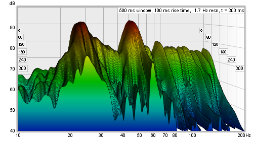
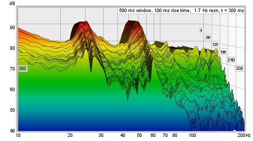
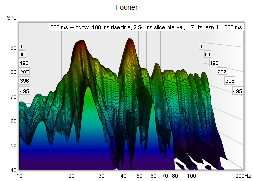
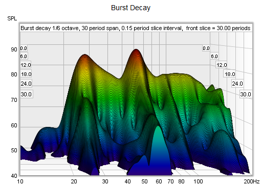
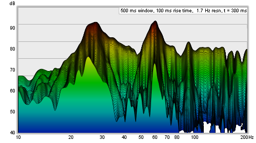
ensures resonances of the same Q decay at the same rate per slice. Here are examples of a Fourier
and Burst Decay waterfall of the same system. The Fourier waterfall spans 500 ms, the Burst Decay
spans 30 periods, which is 500 ms at 60 Hz where the system has a resonance. It is clear from the
Burst Decay that the 60 Hz resonance is higher Q than the 27 Hz resonance.
Right clicking on the graph brings up a menu of actions:
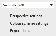
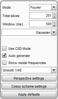
The Smoothing applied to the slices of a Fourier waterfall can be increased from 1/48th octave (the minimum, and recommended) to as high as 1/3rd octave.
The Perspective settings and Colour scheme settings actions bring up the dialogs detailed below.
Export data allows the waterfall slice data to be exported as text.
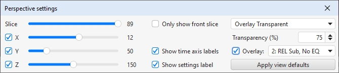
The Slice slider selects which slice is at the front of the plot - as the slider value is reduced the plot moves forward one slice at a time. The trace value shows the SPL figure for the front-most slice, the corresponding time for that slice is shown at the top right of the graph.
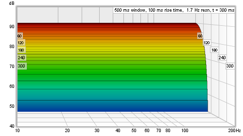
The x, y and z sliders alter the perspective of the plot, moving it left/right, up/down and forwards/backwards respectively. The check boxes next to the sliders allow the perspective to be disabled in that axis. Disabling the x axis can make it easier to see the frequencies of peaks or dips. Disabling the z axis turns off all the perspective effects which makes the plot like a filled spectral decay. Here is the same plot as above but with the x-axis perspective effect turned off.
If Only show front slice is selected only the slice at the front of the waterfall will be shown.
Show time axis labels controls whether the time (or periods) axis grid lines on the sides of the plot are labelled with the corresponding value. Show settings label controls whether to show a label with the plot settings in the top right corner of the plot.
The waterfall allows another measurement's plot to be overlaid on the current measurement. The overlay is generated slice-by-slice, plotting a slice of the current measurement's waterfall, then a slice of the overlay, then the next slice of the current measurement and so on. For this to be possible the waterfalls must cover the same time range and have been generated from measurements with the same sample rate. Overlays are easier to distinguish with the colour scheme set to None. N.B. before a measurement is available to overlay it is necessary to generate the waterfall data for it.
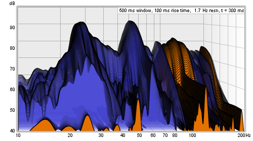
The overlay measurement is chosen from the list of measurements next to the Overlay box, it is shown if the box is selected. Measurements which do not have waterfall data are shown in grey in the selection list. To generate the data for a measurement select it as the current measurement and use the Generate button.
Transparency can be applied to the main plot, the overlay, or both. When transparency is set to 0% both plots are solid. In the image above the main plot is drawn at 75% transparency, allowing the overlay to show through. The transparency mode can be switched between main/overlay/both to ease comparison between the plots.
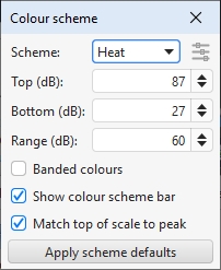
Waterfalls can be generated with the slices filled in the same colour as the measurement or with a colour gradient that varies with SPL. The Scheme selector is set to None to use the measurement colour or to the chosen scheme. Here is an example using the Heat colour scheme:
The Top, Bottom and Range controls adjust how the plot colours correspond to the values in the waterfall data. Any values higher than the Top are drawn in the colour at the top of the scale, any values lower than the Bottom are drawn in the colour at the bottom. If the Top setting is changed the Bottom will be adjusted to keep the same Range. If the Bottom is changed the range will be adjusted to keep the same Top. If the Range is changed the Bottom will be adjusted, keeping the same Top.
If Banded colours is selected the colour scale has discrete steps rather than a continuous blend from one colour to another - there are 11 colours in that case to provide 10 bands across the scale range.
Show colour scheme bar controls whether a bar showing the SPL range of the selected colour scheme is shown to the right of the plot.
Match top of scale to peak adjusts the Top value so that it corresponds to the highest level found in the data.
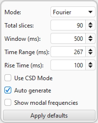
Mode selects the type of spectrogram plot that will be produced, which can be either Fourier or Burst Decay.
The Total Slices control determines how many slices are used to produce the waterfall. Fewer slices mean faster processing and lower memory use, but make it less easy to see how the response is varying. The actual number of slices in a Fourier plot may be up to 20% fewer than the total slices requested to allow the slice interval to be an integer number of samples, which speeds up processing.
The width of the impulse response section that is used to generate a Fourier waterfall is set by the Window control (this control sets the Right Hand window width). The corresponding frequency resolution is shown to the right of the window setting. Longer window settings provide better frequency resolution.
The Time Range control determines how far the impulse response window is moved from its start position to generate the waterfall.
The Rise Time control sets the time duration of the Left Hand window. Shorter settings give greater time resolution but make the frequency variation less easy to see. The default setting, 100 ms, is aimed at revealing room resonances. When examining drive unit or cabinet resonances with full range measurements a much shorter rise time would be used, 1.0 ms or lower, with time spans and window settings of around 10 ms. CSD mode may be more useful for such measurements as the later part of the impulse response can be noisy, obscuring the behaviour in the later slices. The 'rise time' terminology dates back to the late 80s and MLSSA. In MLSSA it referred to the 10% to 90% rise time of a left hand window formed by convolving a window function with a unit step (in essence, the step response of the chosen window function). The actual width of the window was much greater, depending on the window type - about twice the rise time for a Hann window, for example, or about 3 times the rise time for Blackmann-Harris. In REW the term is used to refer to the overall width of the left hand window, somewhat misusing it in the interest of retaining terminology that is in common use for CSD plots whilst adopting a definition that provides a clearer indication of what parts of the response lie inside and outside the chosen window settings. To obtain similar results to the MLSSA-style definition use an REW setting that is twice as long.
Use CSD Mode should be selected if the later slices of the waterfall are contaminated by noise in the measurement. It would commonly be used when examining drive unit or cabinet resonances. CSD mode anchors the right hand end of the window at a fixed point and only moves the left side. This does mean, however, that the frequency resolution reduces (and the lowest frequency that can be generated increases) as the slices progress, as each has a slightly shorter total window width than the previous slice. In CSD mode window width should be greater than the time range (otherwise the window width would be zero at times in the range later than the width of the window).
In Burst Decay mode a Bandwidth control allows burst bandwidths of 1/3rd or 1/6th of an octave to be selected. The 1/3rd octave choice favours time resolution, the 1/6th octave choice favours frequency resolution. With the 1/6th octave burst resonances are more easily distinguished. With the 1/3rd octave burst reflections become more evident in the plot, showing up as curved lines. Burst decay plots may have visible artefacts near the high frequency limit, though typically more than 40 dB below the peak level. A Periods control sets the number of periods the plot will span.
If Auto generate is selected the waterfall will be regenerated automatically if a setting is changed, otherwise new settings will not be applied until the Generate button is pressed.
If Show modal frequencies is selected the theoretical modal frequencies for the room dimensions entered in the Modal Analysis section of the EQ Window are plotted at the bottom of the graph.
Settings can be copied and pasted between measurements by right clicking on the controls panel.
The control settings are remembered for the next time REW runs. The Apply defaults button restores the controls to their default values.
The controls are slightly different for imported audio files. There is no Time Range control, the waterfall is generated for the full range of the imported file. There is no rise time control. A single, centred window is used to generate the waterfall, the window type used is selected from the controls.
Stepped sine measurements have a reduced set of controls and some additional perspective options that are only used for stepped sine data. Each slice in a stepped sine measurement waterfall shows the spectrum data for a test frequency.
The Slice and X, Y, Z perspective controls work in the same way as for sweep measurements. Only show front slice hides all slices except the frontmost, which can be selected using the Slice slider - this is a convenient way to view the spectrum for a single test frequency. The test frequency for the current slice is shown in the top right corner of the graph and on the left and right side walls. Reverse slices switches the order of the slices with the exception of the noise floor, which is the last (frontmost) slice in the set.
Note that waterfalls can only be generated for stepped sine measurements that had the option to Capture spectrum data at each frequency selected.
