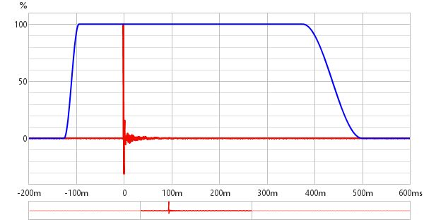
The Impulse graph shows the impulse response for the current measurement. It can also show the left and right windows and the effect of the windows on the data that is used to calculate the frequency response; a minimum phase impulse; the impulse response envelope (ETC) and the step response.
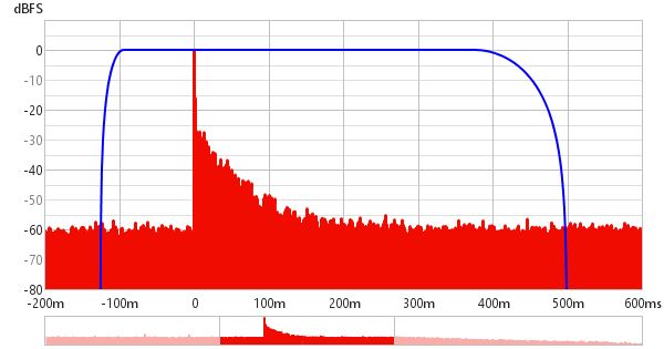
The Y axis used for the impulse response can be selected as % FS or dBFS
(FS = Full Scale) via a control in the top left corner which appears when
the mouse cursor is inside the graph area. The dBFS scale is equivalent to
a "log squared" view of the impulse.

A navigator view below the impulse graph shows the entire response with the currently displayed portion highlighted. The highlighted region can be dragged to reposition the view. Clicking anywhere in the navigator view centres the displayed portion on the click. If the mousewheel is used while the mouse is over the navigator the graph will be zoomed along its time axis, centred on the time axis position of the mouse pointer in the main graph. The navigator replaces the scrollbar, if it is turned off (in the graph controls) the scrollbar will be visible again according to the state of the scrollbars button above the graph.

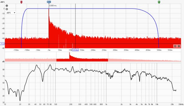
Indicators above the graph show the extents of the impulse response windows and the window reference position. The window settings may be changed by clicking and dragging on the indicators, the new values are applied when the mouse button is released. While the window settings are being changed the region outside the new area is shown shaded until the settings are applied. When the window indicators are dragged a preview of the effect the new setting will have on the SPL response is shown below the impulse response. It is best to set the Y axis to dB to adjust the windows as it is then much easier to see where the response has decayed into the noise.
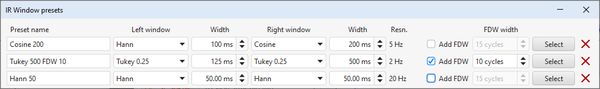
After each measurement the left window width is automatically set up. For full range measurements (and down to end frequencies of 1kHz) the width is 125ms, below that it increases to allow for pre-ringing effects of using a limited sweep range. To change the window settings for a measurement click the IR Windows button:

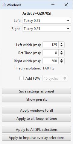
The IR windows dialog allows a set of window presets to be defined which can be created with the Save settings as preset button and applied by selecting them from the presets panel.
The impulse response is that of the whole system, including the mic/meter and the soundcard. The mic/meter and soundcard calibration files are only applied when calculating the frequency response, their effect is not included in the impulse response. However, there is a Merge cal data to IR Measurement action in the All SPL graph controls that allows the cal file responses to be merged into the impulse response.
If the Generate minimum phase control has been used to produce a minimum phase version of the current measurement's magnitude response a minimum phase impulse trace is activated, showing the impulse response the minimum phase system would have. Note that it is necessary to make full range measurements if the minimum phase response is to be generated as a good result relies on measuring beyond the bandwidth of the system being measured.
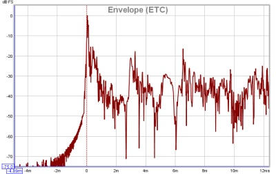
The envelope of the impulse, also called the energy-time curve or ETC, is useful to identify reflections and see the overall shape of the impulse response. The plot below shows the envelope, the spikes after the initial peak are due to reflections from room surfaces, the first spike occurs 3.25ms after the initial peak indicating that the sound travelled an additional 1.11m or 3.7 feet to reach the microphone.
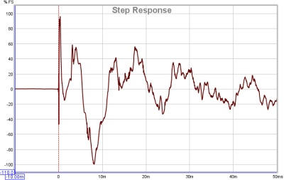
The step response shows the output which would result if the input signal jumped to a fixed level and stayed there. It is the integral of the windowed impulse response. If there is an offset in the measurement input chain the step response will show an overall rise or fall as time progresses, rather than tending back to zero.
A property of the log sweep analysis method is that the various harmonic distortion components appear as additional impulses at negative time, with decreasing spacing as the distortion order increases. For example, this plot shows spikes from distortion components up to the 8th harmonic on a laptop soundcard loopback measurement:
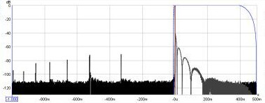
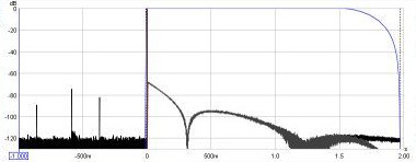
Here is a similar measurement for an external USB soundcard, it is a 44.1k card rather than 48k, which limits us to the 6th harmonic in the 1s pre-impulse period - however, only the 2nd, 3rd and 5th harmonic peaks are evident, the 4th harmonic peak is barely visible above the noise floor (which is about 10dB lower than the laptop card). The extended lobes after the impulse are due to the card's much lower -3dB frequency, 1.0Hz versus 22.1Hz (note that the right side of the time axis is 2.0s in this plot compared to 0.5s in the previous plot):
The Actions panel for the Impulse graph has these actions, there may be more or fewer depending on the measurement type.
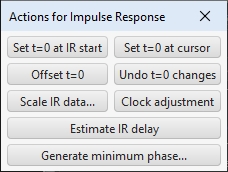
The Set t=0 at IR start button will align the zero position to the time at which the impulse starts (emerges from the noise floor). It can be activated using the Alt+y keyboard shortcut when the controls panel is visible.
The Set t=0 at cursor button will align the zero position to the current cursor position. It can be activated using the Alt+z keyboard shortcut when the controls panel is visible.
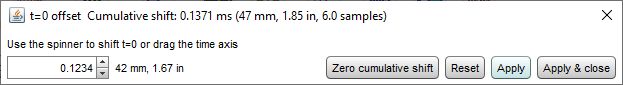
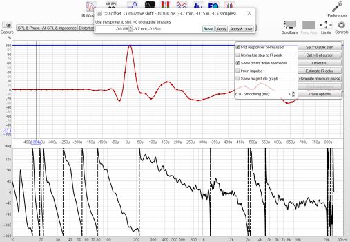
Offset t=0 allows the position of time zero in the impulse response to be altered, with a live preview of the effect the offset will have on phase. The measurement is not changed unless either the Apply or Apply & close button is pressed. Adjustment of the offset can be made by entering a value or by using the up and down arrow keys after clicking on the offset spinner. The cumulative shift that has been applied to the impulse response is shown at the top of the dialog. That includes any shifts applied to the original measured IR to align it to the peak or to the timing reference, if used. The offset can be set to the value required to set the cumulative shift to zero by pressing the Zero cumulative shift button. If a timing reference was used the System Delay figure (which can be viewed in the measurement Info panel) is shifted by the same amount as the zero time.
The Undo t=0 changes button resets t=0 to the as measured state.
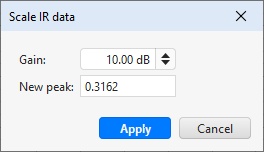
The Scale IR data... button brings up a dialog that allows the impulse response values to be scaled by a chosen gain or to achieve a specified peak value. If the peak value is known type it into the "New peak" field and the gain will be adjusted to suit. The SPL values will not be affected by this action, when the impulse response data is changed a corresponding adjustment is made to the SPL offset.
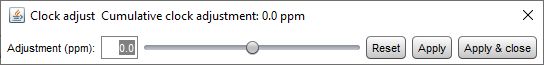
The Clock adjustment control is enabled for log sweep measurements made with REW V5.20 beta 2 or later. It is used to compensate for differences between the clock rates of the output device and input device. When the output and input device are different their clocks may differ sufficiently to distort the shape of the impulse response, particularly when using longer sweeps. The clock rate difference affects the phase response (magnitude is not affected). The adjustment is in units of parts per million, ppm. While the clock rate is being adjusted a live preview shows the effect the adjustment will have on the impulse response and phase. The measurement is not changed unless either the Apply or Apply & close button is pressed. Fine adjustment can be made with the left and right arrow keys after clicking on the slider knob. The control has a range of -500 to +500 ppm, but greater adjustments can be made by using the Apply button then applying further changes as required. The cumulative clock adjustment is shown at the top of the dialog and in the measurement Info dialog. Note that clock adjustment is a computationally intensive task so the display updates are not immediate.
Generate minimum phase will produce a minimum phase version of the measurement using the current IR window settings. The minimum phase impulse then shows the response of a system having the same frequency response as the measurement but with the lowest phase shift such a system could have. Note that it is best to make full range measurements if the minimum phase response is to be generated as a good result relies on measuring beyond the bandwidth of the system being measured. This control also activates minimum and excess phase and group delay traces on the SPL & Phase and GD graphs respectively.
Note that the IR window settings are important as the minimum phase response is derived from the frequency (magnitude) response of the measurement, which in turn is affected by the IR window settings. If the window settings are subsequently changed Generate minimum phase should be used again to reflect the new settings. Note also that the shape of the left side window (the window applied before the peak) affects the minimum phase result, a rectangular window will produce a response with lower phase shift than, for example, a Hann window.
If the system being measured was inherently minimum phase (as most crossovers are, for example) the minimum phase response is the same as removing any time delay from the measurement. Room measurements are typically not minimum phase except in some regions, mainly at low frequencies. For more about minimum and excess phase and group delay see Minimum Phase.
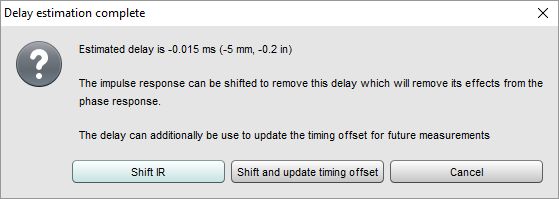
Estimate IR delay (Ctrl+Alt+E) calculates an estimate of the time delay in the measurement by comparing it with a minimum phase version. The delay it calculates can be removed from the impulse response by pressing the Shift IR button on the panel shown after the delay is calculated and can additionally be applied as a timing offset for subsequent measurements.
The control panel for the Impulse graph has these controls:
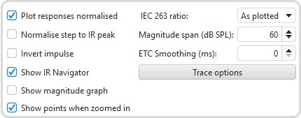
The impulse response may be plotted with or without normalisation to its peak value according to the setting of the Plot responses normalised control. When normalised plotting is selected the peak will be at 100% or 0 dBFS.
The step response may be normalised to its own peak value or to the peak value of the impulse response according to the setting of the Normalise step to IR peak control.
The impulse response may be inverted according to the setting of the Invert impulse control. Note that this has no effect on the displayed impulse response when the Y axis is set to dBFS. If the soundcard you are using inverts its inputs that can be corrected using the Invert checkbox in the Soundcard Preferences Input Channel controls.
If Show IR Navigator is selected the navigator view is shown below the graph.
If Show magnitude graph is selected the response SPL graph is shown below the impulse graph. The view is the same as that shown when adjusting the IR windows using the indicators at the top of the graph. The IEC 263 ratio control sets the aspect ratio of the magnitude graph, Magnitude span (dB SPL) sets its SPL span.
If Show points when zoomed in is selected the individual points that make up the response are shown on the graph when the zoom level is high enough for them to be distinguished.
The IEC 263 ratio control allows the magnitude graph to be locked to a specified dB/decade aspect ratio. The aspect ratio is maintained by adjusting the margins around the graph as required.
The Magnitude span (dB SPL) control sets the Y axis span of the magnitude graph.
ETC Smoothing is used to smooth the envelope (ETC) trace using a moving average filter of the duration specified in the spinner.
The Trace options button brings up a dialog that allows the colour and line type of the graph traces to be changed. If a change is made it will be used for all measurements shown on this graph. Traces can also be hidden, which will remove them from the graph and from the graph legend.