To make sense of the measurements you can take with REW it is helpful to have an understanding of what the measurements are. This topic gives an overview of the basics of signals and measurements and explains how the various graphs in REW are generated and how they relate to what we have measured.
The first thing to understand is what a signal is, at least in the context of making acoustic measurements. The signals we are interested in are sounds recorded through a microphone or SPL (Sound Pressure Level) meter. The sound pressure generates electrical signals in the mic/meter which are captured by our audio interface. The interface takes measurements of the electrical level at its input. Each measurement is referred to as a sample. How often it takes its samples is controlled by the sample rate. REW supports a range of sample rates depending on the capabilities of the interface, common rates are 44.1kHz or 48kHz - which means the interface is capturing the level at its input either 44,100 or 48,000 times every second. Three seconds of a signal sampled at 48kHz means a sequence of 3*48,000 = 144,000 measurement values. The highest frequency that can be captured at any given sample rate is half the rate - we need at least two samples for each cycle of the frequency to reproduce it. At 48kHz sampling that means the highest frequency we can capture is 24kHz. Frequencies higher than half the sample rate would cause aliasing, they would appear to be lower than they actually were. For example, a 25kHz signal sampled at 48kHz would actually look like a 23kHz signal. To prevent this, the inputs of the interfaces have anti-aliasing filters that try to block signals higher than can be captured, but they are not completely effective so we always need to consider the frequency content of the signals we are trying to capture.
The resolution of the interface measurements is typically either 16 bits or 24 bits. 16 bit resolution is the same as used on CDs, and is the resolution REW supports. Having 16 bit resolution means the individual measurement values can range from -32768 to +32767 (numbers that can be represented with 15 binary digits, plus a 16th binary digit to store the sign of the number). Rather than use the measurement numbers directly, it is convenient to refer to them in terms of how close they are to the largest number, which is referred to as Full Scale and abbreviated as FS. The full scale values are -32768 and +32767. The smallest non-zero measurement value is 1, which as a percentage of full scale is 100*(1/32768) or approximately 0.003% FS. Anything smaller than that is seen by the interface as zero. The full scale value will correspond to a certain voltage at the interface input - that is usually around 1 Volt. Soundcards that have higher resolution, such as 24 bit, usually have the same maximum input voltage (around 1 Volt) but can use a wider range of numbers to measure the voltage. For a 24-bit interface the full scale measurement values are -8388608 and +8388607. That still is only 1 Volt (typically), the largest input voltage has not changed, but the 24-bit interface has higher resolution - the smallest value it can detect is 100*(1/8388608) percent of full scale, 0.000012% FS. It is with the very smallest signals that higher resolution has benefits. The full scale value is often treated as corresponding to a value of one, and everything below full scale as being the corresponding proportion of one, so half full scale would be 0.5 and so on.
If the signal gets larger than the full scale value the interface is unable to follow it - the measurement value cannot get higher than full scale no matter what is actually happening at the input. When the signal has gone beyond the range the input can measure it is said to have been clipped. Clipping shows up in input signals as flat parts of the response. If the clipping happens at the interface input it will be at +100% FS or -100% FS and REW will warn you, but sometimes clipping can happen before the signal gets to the interface (in a mic preamp whose gain is set too high, for example). In that case the measurement values may never reach the interface's FS levels but the signal is clipped nonetheless. Clipping must be avoided when measuring, because the captured signal no longer represents what was actually happening at the input and that corrupts the measurement.
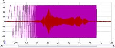
One way to look at signals is to plot the measurement values against time. When captured
signals are plotted in REW on the Captured graph they are shown as % FS, a
signal that reaches 100% FS is the largest the interface can capture. An example of an REW
Scope plot is shown below, displaying a sweep signal REW has generated and (in red) the resulting
signal captured from a microphone.
We are usually interested in more than just the sample values. The frequencies that make up the signal may also be of interest. The range of frequencies that make up a signal is called its Spectrum and we can calculate them using a Fast Fourier Transform or FFT. The FFT works out the amplitudes and phases of a set of cosine waves that, when added together, would give the same set of measurement values as the time signal. The amplitudes and phases of those cosine waves are a different way of representing the time signal, in terms of the frequencies that make it up rather than its individual measurement values. The amplitudes are easy to understand, a larger amplitude means a bigger cosine wave. The phases indicate the starting value for the cosine waves at the time of the first sample in the sequence that was measured. A phase of zero degrees would mean the starting value was amplitude*cos(0) = amplitude. A phase of 90 degrees would mean a starting value of amplitude*cos(90) = 0. We are more often interested in the amplitudes than the phases, but we shouldn't forget about the phases entirely - they contain half the information about the shape of the original time signal.
When an FFT is used to calculate the spectrum it uses a set of frequencies that are evenly spaced from DC (zero frequency) up to half the sample rate (the maximum that can be properly represented). The spacing depends on the length of signal we analyse in the FFT. FFT calculations are most efficient when the signal lengths are powers of two, such as 16k (16,384), 32k (32768) or 64k (65536). To calculate a 64k FFT from a signal that is sampled at 48kHz we need 65536/48000 seconds of the signal, or 1.365s. The frequencies would be spaced at 24000/65536 = 0.366Hz. If the FFT were generated from 16k samples the frequencies would be 1.465Hz apart. The fewer samples used to generate the FFT, the further apart the frequencies are so the lower the frequency resolution. For high frequency resolution we need to analyse long time periods of signals.
A common way of viewing the spectrum of a time signal is to use a Real Time Analyser or RTA.
The RTA shows a plot of the amplitudes of the frequencies that make up the signals it is analysing.
However, whereas the FFT produces signals that are at uniformly spaced frequencies, an RTA groups
them together in fractions of an octave. An octave is a doubling of frequency, so the span from
100Hz to 200Hz is one octave. So is the span from 1kHz to 2kHz - the actual frequency span of an
octave fraction is more the higher the frequency gets. For a 1/3 octave RTA the span is about 4.6Hz
at 20Hz, but is 4.6kHz at 20kHz. For a 1/24 octave RTA the spans are 1/8th as wide. Within the span
of an octave fraction many individual FFT values may be used to produce the single value the RTA
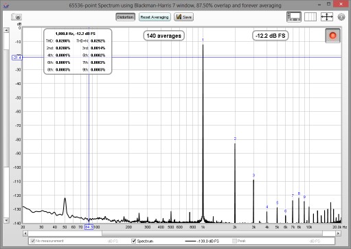
assigns to that band of frequencies. Below is an image of the REW RTA displaying the spectrum of
a 1kHz tone and its distortion harmonics.
Viewing the spectrum of a signal has its uses, but we are also interested in how the equipment we use alters the spectrum of signals. The way a system changes the spectrum of signals that pass through it is called the system's Transfer Function. The transfer function has two components, the Frequency Response and the Phase Response. The frequency response shows how the amplitudes of frequencies are changed by the system, the phase response shows how the phases of frequencies are changed. A complete description of the system needs both responses, very different systems can have the same frequency response but their different phase response lets us distinguish them.
Note that it is important not to confuse a system's frequency response with the spectrum of
the system's output. The spectrum of a signal shows us what that signal is made up of in terms
of the frequencies it contains. The transfer function's frequency response tells us how the
system changes the spectrum of signals. The purpose of measurement software like REW is
to measure transfer functions, and REW's SPL & Phase graph shows the transfer function's
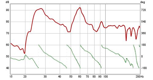
frequency and phase responses. The frequency response amplitude is shown as an SPL trace. Below
is a plot of the frequency response (upper trace, left hand axis) and phase response (lower trace,
right hand axis) from a room measurement, showing the span up to 200Hz.
The transfer function shows us, through the frequency and phase responses, how the system
affects the spectrum of signals that pass through it. It characterises the system in what is
called the frequency domain. But what about the signal itself? How do we describe
how the individual samples of the signal are changed by the system, its time domain
behaviour? The way a system changes the samples of a signal is called its impulse response.
The reason for the name will become clear. The impulse response (IR) is
itself a signal, consisting of a series of samples. Signals that are input to the system overlap
the IR as they pass through, sliding along it sample by sample. When the signal first appears,
its first sample lines up with the first sample of the impulse response. The system output
for that first input sample is the first IR sample value multiplied by the first signal sample
value:
output[1] = input[1]*IR[1]
One sample interval later, the input has a 2 sample overlap with the IR. The output for this
time period is the 2nd input sample times the first IR sample, plus the first input sample times
the second IR sample:
output[2] = input[2]*IR[1] + input[1]*IR[2]
Another sample period later the input overlaps the IR by 3 samples, the output is
output[3] = input[3]*IR[1] + input[2]*IR[2] + input[1]*IR[3]
And so it goes on, as each successive input sample appears. That process of multiplying input
signal samples by IR samples is called convolution. Typically the impulse response has
a fairly short duration, much less than a second for a measurement of a piece of equipment and a
second or two for a measurement of a domestic-sized room, so eventually the output at each time
period consists of the length of the IR multiplied by the same length of the input signal, with
all the individual products added up to give the output for that time period.
What output would we get if the input signal consisted of a single sample at full scale, to which
we will assign a value of one, followed by zeroes for all other samples? The initial output sample
would be
output[1] = input[1]*IR[1] = IR[1]
The next output sample would be
output[2] = input[2]*IR[1] + input[1]*IR[2] = 0*IR[1] + 1*IR[2] = IR[2]
The third sample would be
output[3] = input[3]*IR[1] + input[2]*IR[2] + input[1]*IR[3] = 0*IR[1] + 0*IR[2] + 1*IR[3] = IR[3]
and so on. The output would consist of each sample of the IR in turn. An input that has just a
single full scale sample followed by zeroes is called an impulse, so the output of the
system when fed that input is called the impulse response.
As the transfer function and the impulse response are both descriptions of the same system we might reasonably expect that they are related, and they are. The transfer function is the FFT of the impulse response, and the impulse response is the inverse FFT of the transfer function. They are both views of the same system, one in the frequency domain and the other in the time domain. The transfer function is simply the spectrum of the impulse response.
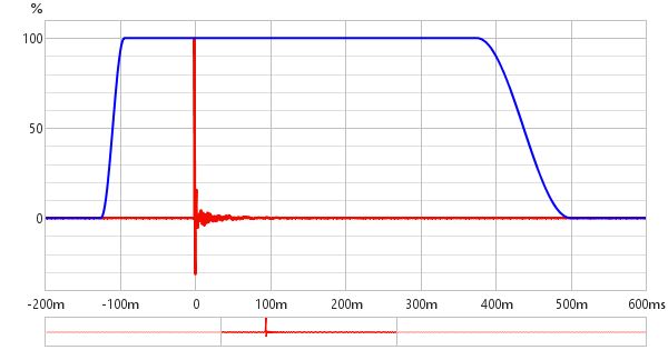
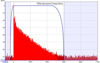
The REW Impulse graph displays the impulse response. It shows the values as either % FS
or dBFS. The dB scale is useful to see a wider dynamic range of the signal, rather
than plot the values directly it plots the base 10 log of the values multiplied by 20. The top
of the dB plot is 0 dBFS, which corresponds to 100% FS. A level of 50% FS would be 20*log(0.5) =
-6 dBFS. 10% FS is 20*log(0.1) = -20 dBFS. The dBFS scale is useful to see how the lowest levels
of the impulse are behaving and where it gets lost below the noise level of the measurement. The
images below show an impulse response with % FS as the Y axis then the same response using dBFS.
In the second image we can see the impulse takes longer to decay into the noise floor of the
measurement than it might seem from the % FS plot.
The system we want to measure might be a piece of equipment, like a loudspeaker, but in acoustics the system we are actually measuring includes other equipment and environments in the path between the signal generated for the measurement and the signal picked up for analysis. These include amplifiers, the microphone, the interface and most importantly the room itself. The system we are actually measuring includes all those elements, so to focus on one part of it we will need ways of removing the influence of the parts we are not interested in.
The response of the interface can be calibrated out by measuring it separately, as can the response of the microphone. Removing the effect of the room is more difficult. It may be the effect of the room is what interests us, especially if we are studying what we are hearing at our listening position, but if we are trying to isolate the performance of a loudspeaker the room's contribution can obscure details of the loudspeaker's performance.
The signal that reaches the microphone travels along a direct path, which is the shortest route from the loudspeaker and so takes the shortest time. The sound from the loudspeaker also radiates outwards and bounces off the room's surfaces. The reflections from those surfaces travel further before they reach the microphone, so they take longer to arrive. If the signal was an impulse, we would expect to see the direct arrival first, then the arrivals from the reflections. Those later arrivals are delayed by the extra time taken to travel the additional distance. The shortest that extra time can be is the time it takes sound to travel to the nearest surface - if that nearest surface was 3 feet away, for example, it would take at least 3 milliseconds longer for a reflection from that surface to reach the mic than the direct sound from the speaker (in practice it would take a little longer than that as the path distance would be a little more than 3 feet).
If we were to examine just the first few ms of the impulse response we would see the part that corresponds to the initial arrival, which came directly from the loudspeaker without a contribution from the room. Looking at a small portion of the impulse response in that way is called windowing the response (in the impulse response images a few paragraphs above the blue trace shows the window). If we calculate an FFT for that windowed portion of the IR we can see the transfer function for that direct arrival, which would be the transfer function of the loudspeaker alone. There is a drawback, however. If we take the FFT of a short signal, we can only see the response down to a limit that depends on how long the signal was. If we had a whole second of signal we can get a frequency response that goes down to 1Hz. If we only had 1/10th of a second, we only get a frequency response that goes down to 10Hz. In general, if the length of signal we analyse is T seconds, the lowest frequency is 1/T - so if our window was only 3ms long, the frequency response would only go down to 1/0.003 = 333Hz. To see low frequency responses free of room influences the nearest surface needs to be as far away as possible. To adjust the window settings in REW click the IR Windows button. By default REW uses window settings that include more than 0.5s of the impulse response, so that the effect of the room can be seen.
The SPL & Phase and Impulse graphs are the most useful for studying the transfer
function we have captured, but there is another graph that gives us useful information about
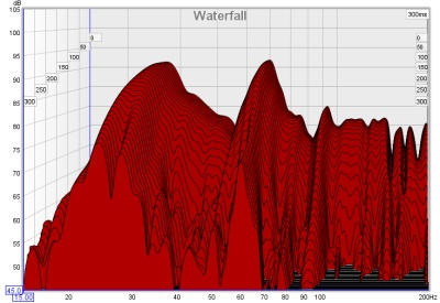
what the room is doing to the sounds we play in it. That graph is the Waterfall. The
waterfall is a plot of how the spectrum of a section of the impulse response changes as time
progresses. It is produced by windowing an initial part of the response, typically a few hundred
ms when looking at room responses, and calculating an FFT of that windowed section. The FFT
produces the first slice of the waterfall. We then move the window along the impulse response
a little and calculate another FFT to produce the second slice of the waterfall. Moving the
window along a little further gives us the third slice, then the fourth and so on. As we move
further along the waterfall we start to lose the initial contribution from the loudspeaker and
increasingly see just the contribution of the room. The room's response is strongest at
frequencies where there are modal resonances, which are frequencies at which the sound
bouncing back and forth between the room's surfaces reinforces itself to produce stable, slowly
decaying tones. Those frequencies stand out as ridges in the waterfall plot, with the worst
modal resonances having the highest ridges that take the longest to decay.
That was a very quick introduction to the basic signal and measurement concepts. If you have stuck with it all the way to the end, well done. Now you have the information needed to better understand how REW makes measurements.