The RTA window allows Real Time Analyser (RTA) or spectrum analyser plots
to be generated, updating as the input signal is analysed. It is shown
by pressing the RTA button in the toolbar of the main REW window.
![]()
The RTA trace is activated by pressing the record button
![]() in the top right hand corner of the graph area, after which it will continuously
analyse blocks of input samples and display the frequency spectrum of each block. If the
RTA settings are such that the update interval is more than 1 second the record button
will show a percentage progress figure.
in the top right hand corner of the graph area, after which it will continuously
analyse blocks of input samples and display the frequency spectrum of each block. If the
RTA settings are such that the update interval is more than 1 second the record button
will show a percentage progress figure.
Sometimes the analyser is used without a test signal, for example to look at the frequency content of background noise, but more often it is used together with the REW generator or an external generator or signal source. If the generator is playing a pink noise signal (or even better, pink Periodic Noise) the RTA display will show the frequency response of the room, updated live so that the effects of changing EQ settings can be immediately seen.
Playing a sine wave test tone on the generator allows the levels of the tone and its harmonics to be observed on the analyser and distortion percentages to be calculated, whilst using the dual tone generator allows intermodulation distortion measurements.
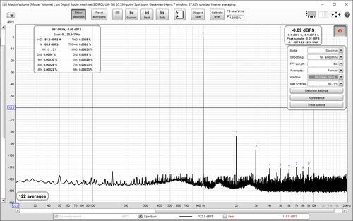
The RTA plot shows the currently selected measurement as a reference and the live RTA or spectrum. A Peak trace is also available, which is reset by the Reset averaging button. If Inverse C compensation is being applied the icon is shown after the trace value. If Mic/Meter calibration file or soundcard calibration file have been loaded they are applied to the results.
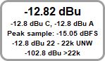
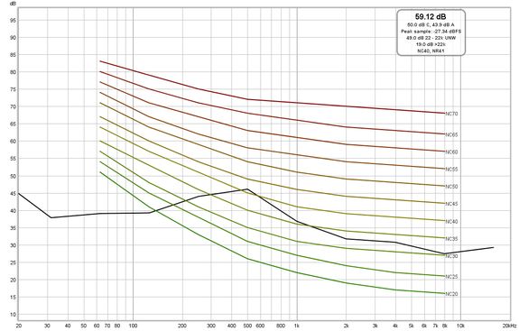
The current Input RMS value is shown to the left of the record button, in dB SPL, dBFS, dBu, dBV, dBW, volts or watts according to the setting of the Y axis. This figure excludes any DC content in the signal. A and C weighted values are shown below the unweighted rms figure. All three figures are calculated over the range specified by the distortion LP and HP settings, if either or both are enabled. The peak sample value in the last RTA block is shown in dBFS. Below that are the in-band (22.4 Hz to 22.4 kHz) and, for sample rates above 44.1 kHz, out of band (> 22.4 kHz) unweighted RMS levels. If clipping is detected in the input the RMS value turns red. If the RTA is in one octave mode Noise Criterion and Noise Rating figures will be shown below the RMS values.
A dBc Y axis option is offered which places the peak level of the input at 0 dBc, or places the peak of the fundamental at 0 dBc when the distortion panel is active. There is also a volts per √Hz Y axis option to display the amplitude spectral density, this is only meaningful when using the spectrum view.
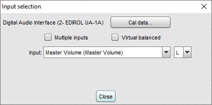
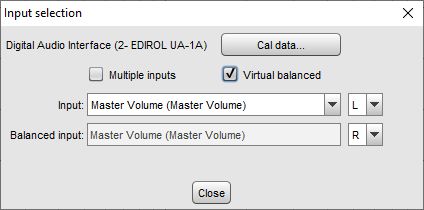
The current RTA input can be changed by clicking the Input selection button:
![]()
That brings up an input selection dialog, which also has a button to show the currently
active mic cal data.
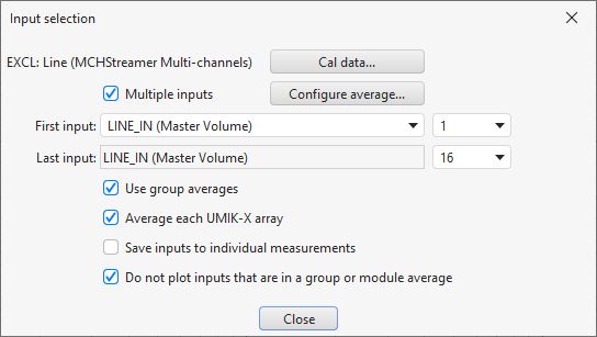
When using multi-input capture (Pro upgrade) there is an option to select multiple inputs and choose the range of inputs that will be averaged by the RTA to produce the graph traces. Up to 16 individual input traces can be displayed along with the average and peak, according to the setting in the View preferences. Weighting and SPL alignment can be configured before or during capture using the Configure average button.
Multi-input RTA measurements are saved in the same format as multi-input sweep measurements allowing the same weighting and SPL alignment adjustments to be made to them after measurement have been captured. If the Save inputs to individual measurements option is selected saving the current input will produce a measurement for the average and individual measurements for each input channel.
If only two inputs are selected for a multi-input RTA measurement distortion and levels will be shown individually for each.
If the Virtual balanced input option is selected a Balanced input selection is offered. The balanced input will be subtracted from the measurement input and the result scaled by 0.5. This simulates the behaviour of a balanced input, and is appropriate if the balanced input is driven by an inverted signal (such as by selecting the Invert second output option on the signal generator.
The input level for the current measurement input channel can be calibrated by pressing the Calibrate level button above the graph while the RTA is running. A signal with a known rms voltage level should be applied to the input and that rms level entered in the calibration dialog.
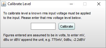
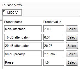
After the value is entered a confirmation message will be shown, stating the maximum peak and rms input voltages the input can accept before clipping at digital full scale. If any volume control setting along the input path is altered the calibration will need be done again. If the input sensitivity is known (including the effect of any volume control settings) it can be typed directly into the text field below the FS sine Vrms label. Clicking in the triangle in the upper left corner brings up a list of preset values that may be entered, the labels and values can be changed as required.
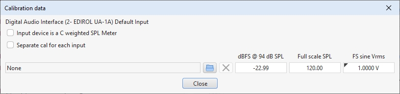
The full scale input level can also be entered by using the Cal data button on the
input selection dialog to bring up the cal data settings which has a field labelled FS sine Vrms.
The level is saved as part of the calibration data for the input device and will be used whenever that
input device is selected on the Soundcard preferences.
The Save current button converts the current display into a measurement in the measurements pane (keyboard shortcut Alt+S). It is converted in the current mode of the analyser, so if the analyser is in Spectrum mode the measurement shows the spectrum, if it is in RTA mode it shows the RTA result. The saved measurements can be used as references for subsequent spectrum/RTA measurements. If distortion data is available it is copied to the comments area of the saved measurement. Peak data can similarly be saved using the Save peak button, or both saved at once using the Save both button.
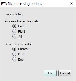
The RTA can be used to analyse WAV files (singly or in groups) by dragging and
dropping them on the RTA window or by clicking the Open WAV button (shortcut Alt+O) to
select a WAV file to process. The dialog below appears to determine how each file will
be processed, at the end of processing the current, peak or both results will be
saved as measurements according to the selection made.
The controls for the plot are shown below.
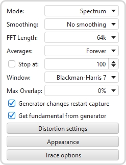
The Mode can be set to Spectrum for a spectrum analyser plot or to various RTA resolutions from 1 octave to 1/48 octave. The difference between spectrum and RTA modes is how the information is presented. In spectrum mode the frequency content of the signal is split up into bins that are all the same width in Hz. For example, with a 64k FFT length and 48 kHz sample rate the bins are 0.732 Hz wide. The plot shows the energy in each of those bins. In RTA mode the bin widths are an octave fraction, so their width in Hz varies with the frequency. For example, a 1 octave RTA plot has bins that are 70.7 Hz wide at 100 Hz (from 70.7 Hz to 141.4 Hz) and 707 Hz wide at 1 kHz (from 707 Hz to 1.414 kHz). The plot shows the combined energy at each frequency within each bin. This is closer to how our ears perceive sound. The different presentations mean signals with a spread of frequency content will look different on the plot. The best known examples are white noise and pink noise. White noise has the same energy at each frequency. On a spectrum plot, which shows the energy at each frequency, the white noise plots as a horizontal line. On an RTA plot it appears as a line that rises with increasing frequency, as each RTA bin gets wider it covers more frequencies and so has more energy. The bin widths double with each doubling of frequency so the energy also doubles, which adds 3 dB on the logarithmic plots we use to show level. White noise sounds quite 'hissy', we perceive it as having more energy at higher frequencies.
Pink noise has energy that falls 3 dB with each doubling of frequency. On a spectrum plot it is a line that falls at that 3 dB per octave rate, on an RTA plot it is a horizontal line as the energy in the signal is falling at the same rate as the bins are widening. We perceive pink noise as having a uniform distribution of energy with frequency.
Single tones are a special case, they will appear at the same level on either style of plot as their energy is all at one frequency, so on a spectrum plot they show as a vertical line, on an RTA plot they show (typically) as a bar of the width of the bin at their frequency, but the height of the bar is the same as the height of the line on the spectrum as all the energy is at that one frequency.
Smoothing can be applied to the trace according to the setting of the Smoothing box.
The FFT Length determines the basic frequency resolution of the analyser, which is sample rate divided by FFT length. The shortest FFT is 8,192 (often abbreviated as 8k) which is also the length of the blocks of input data that are fed to the analyser. An 8k FFT has a frequency resolution of approximately 6Hz for data sampled at 48kHz. As the FFT length is increased the analyser starts to overlap its FFTs, calculating a new FFT for every block of input data. The degree of overlap is 50% for 16k, 75% for 32k, 87.5% for 64k and 93.75% for 128k. The overlap ensures that spectral details are not missed when a Window is applied to the data. The maximum overlap allowed can be limited using the Max Overlap control below to reduce processor loading at higher FFT lengths.
The plot can be set to show the live input as it is analysed or to show the result of averaging measurements, according to the selection in the Averaging control. Selecting a number for averages results in that many measurements being averaged to produce the result, with the oldest measurement being removed from the average as each new measurement is added. There are several Exponential averaging modes, which give greater weighting to more recent inputs. The figure shown in the selection box is the proportion of the old value which is retained when a new measurement is added, the higher the figure the more heavily averaged the display becomes. There is also a Forever averaging mode which averages all measurements with equal weight since the last averaging reset. In Forever averaging the Stop at option allows the RTA to be stopped when a configured number of averages is reached. After starting the RTA or changing the FFT length averaging does not begin until a full FFT length of data has been received, plus the lengths of the input and output buffers.
The Reset averaging button above the graph restarts the averaging process (keyboard shortcut Alt+R). If the signal generator is started or is running and its settings are changed while using the RTA the averaging will be automatically reset. Averaging is needed when measuring with pink noise or when there is noise in the signal being measured. Note that if measuring a response using pink noise the best results are obtained using REW's periodic noise signals, which can be exported as wave files from the signal generator to produce a test disc for the system to be measured if direct connection to the PC running REW is not possible.
The FFT resolution is also affected by the Window setting. Rectangular
windows give the best frequency resolution but are only suitable when the signal
being analysed is periodic within the FFT length or if a periodic noise signal is being
measured. The Rectangular window should always be used with the REW
periodic noise signals.
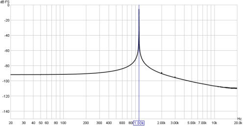
Most other signals, e.g. sine waves from the REW generator or test tones on a CD or random noise,
typically would not be periodic in the FFT length. Using a rectangular window when
analysing such a tone would generate spectral leakage, making it difficult to resolve
the frequency details - the plot below shows an example of a 1kHz tone from an
external generator with a Rectangular window.
Here is the same tone analysed with a Hann window.
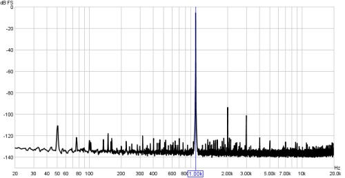
The window allows the harmonics of the tone to be resolved.
However, the tradeoff is that windows cause some spreading of the signal they
are analysing, which reduces the frequency resolution. To use a rectangular window
with the REW signal generator use the generator's
Lock frequency to FFT option.
The Hann window is well suited to most measurements, offering a good tradeoff between resolution and shoulder height. If very high dynamic range needs to be resolved (very small signals close to very large signals) use the 4-term or 7-term Blackman-Harris windows. If the spectral peak amplitudes must be accurately measured use the Flat Top window, this will provide amplitude accuracy of 0.01 dB regardless of where the tone being measured falls relative to the bins of the FFT. The other windows only show the spectral amplitude accurately if the tone is exactly on the centre of an FFT bin, if the tone falls between two bins the amplitude is lower, with the maximum error occurring exactly between two bins. This maximum error is 3.92dB for the Rectangular window, 1.42dB for Hann, 0.83dB for the 4-term Blackman-Harris and 0.4dB for the 7-term Blackman-Harris.
The spectrum/RTA plot can be updated for every block of audio data that is captured from the input, overlapping sequences of the chosen FFT length. This can present a significant processor load for large FFT lengths. The processor loading can be reduced by limiting the overlap allowed using this control.
If Generator changes restart capture is selected RTA capture will restart if the signal generator is started or is running and its settings are changed while using the RTA.
If Get fundamental from generator is selected the fundamental frequency will be obtained from the generator if the generator is playing a sine tone, otherwise it will be determined from the largest peak in the input. Getting the fundamental frequency from the generator ensures accurate determination of harmonic frequencies even if heavy distortion causes the fundamental to have an asymmetric spectrum. It is also required if an external notch filter is used to remove the fundamental. On the other hand, if the system DAC and ADC have different clock sources (e.g. if they are different devices) the received frequency (based on the ADC clock) may differ sufficiently from the generated frequency (based on the DAC clock) to misidentify harmonics, particularly for very long FFTs. In that case the option should not be selected and the RTA will show a warning.
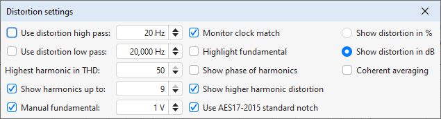
The Distortion High Pass and Low Pass are used to set the lowest and highest frequencies that will contribute to the calculation of THD, THD+N and, for dual, triple and multitone signals, TD+N. They are only applied when the Use distortion high pass and Use distortion low pass boxes are selected. Either can be enabled individually. When they are active the region of the plot which is excluded from the calculations will be greyed out and the THD, THD+N and TD+N figures will show the range over which they have been calculated.
A value for the fundamental level may be entered for use in harmonic distortion calculations when the fundamental is attenuated by a notch filter. The level is in Vrms and should take account of any gain introduced after the notch. That ensures REW uses the correct fundamental level when calculating distortion. To compensate for the effect of the notch filter on harmonic levels its response can be loaded as a calibration file. For example, make a sweep measurement of a loopback connection firstly with the notch filter in place, then another without it, then use the Trace arithmetic feature of the All SPL graph to generate (notch response)/(no notch response) and export that result as a text file to be loaded as a mic cal file. Alternatively just measure the notch response, offset the measurement so that the dB values correctly reflect the notch filter loss at the harmonics (the fundamental is not critical since Manual fundamental deals with that) and export that offset notch response as text and load it as the mic cal file. The harmonic levels will then be corrected to allow for the filter's attenuation. The fundamental levels shown by the graph trace will typically be in error due to shifts in the centre frequency of the notch, but they will not be used if Manual fundamental is selected.
Distortion ratios may be shown as either percentages or in dB according to the selection made.
The Highest harmonic in THD setting controls which harmonics are used for the calculated THD figure. The THD figure in the distortion panel will show which harmonics are included. Note that this has no effect on THD+N, only on THD.
If the Show harmonics up to option is selected the distortion data panel
shows the levels of harmonics up to the figure in the adjacent box. If the
Show phase of harmonics option is selected the distortion data panel
includes the phase of each harmonic relative to the fundamental. If
Show higher harmonic distortion is selected a figure is shown for harmonics
from the tenth up to the highest within the measurement bandwidth, with an upper limit
of the 50th.
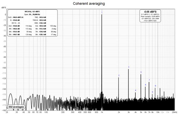
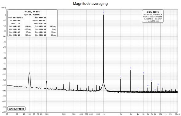
This option is only applicable to harmonic distortion measurements and only when capturing a single input. If it is selected the FFT data is phase aligned according to the phase of the fundamental before averaging, this can lower the noise floor substantially compared to magnitude averaging without needing very long FFTs - in fact shorter FFTs (e.g. 64k) will allow faster averaging and more quickly lower the noise floor. The noise level drops by about 3 dB for each doubling of the number of averages. Mains frequency components will be suppressed along with any other noise not harmonically related to the fundamental, so this option is only suitable for examining harmonic levels. Note that if the harmonic levels are varying coherent averaging will converge to their average level whilst magnitude averaging will converge to their rms level. The various noise-related values in the distortion panel (THD+N, N, N+D) continue to be calculated from magnitude-averaged data and remain valid.
If the Use AES17-2015 standard notch option is selected the fundamental power for THD and THD+N calculations will be the power within a one octave span around the fundamental frequency. If that option is not selected it will be the power in the main lobe of the fundamental. When the fundamental level is not well above the noise floor using the standard notch will produce a higher figure than the fundamental main lobe, in those cases it is better not to use the standard notch setting.
If the Monitor clock match option is selected REW will check for differences between the replay and record clock rates when using a multitone test signal or an FFT-locked sine signal and warn if the clock rates do not match and a rectangular window should not be used. If the window is not rectangular and the clock rates do match it will suggest using a rectangular window for greatest accuracy in the results.
If the Highlight fundamental option is selected the portion of the response which contributes to the fundamental power for THD and THD+N calculations will be highlighted. The response outside the highlighted region is used for the noise and noise+distortion calculations.
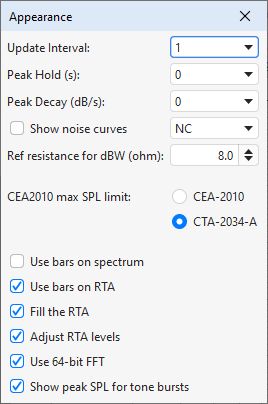
The spectrum/RTA plot is updated by default for every block of audio data that is captured from the input. This can cause a significant processor load, particularly if the RTA window is very large or for large FFT lengths. The processor loading can be reduced by updating the plot less often, which is set by the Update Interval control. An update interval of 1 redraws the trace for every block, an interval of 4 (for example) only updates the trace on every 4th block.
The Peak Hold and Peak Decay controls set how long, in seconds, a peak value is held and how quickly, in dB per second, the peak values decay. If Peak Hold is set to 0 the peak values are not held at all. If Peak Decay is set to 0 the peak trace does not decay.
If the Show noise curves option is selected when capturing a single input the chosen noise curves will be drawn on the graph when the RTA is in 1 octave mode and the Y axis is showing dB. The options are Preferred Noise Criterion (PNC), Balanced Noise Criterion (NCB), Noise Criterion (NC) and Noise Rating (NR). Note that if Adjust RTA levels is selected the curves will be offset by the same amount as the RTA trace, but this will not alter the noise criteria results.
The watt and dBW values are calculated from the voltages assuming a reference load resistance, this control sets the value of that resistance.
The thresholds for distortion plus noise when using the CEA2010 burst test signal can be selected as those used for the ANSI/CTA-2010-B R-2020 Standard Method of Measurement for Powered Subwoofers or the ANSI/CTA-2034-A Standard Method of Measurement for In-Home Loudspeakers. The colour of the threshold overlay reflects the corresponding band chosen according to the fundamental frequency, per the standards.
In Spectrum or RTA modes the plot can either draw lines between the centres of the FFT bins or draw horizontal bars whose width matches the FFT bin or RTA octave fraction width, this is controlled by the Use bars on spectrum and Use bars on RTA check boxes.
In RTA mode the plot will be filled if Fill the RTA is selected.
The RTA plot shows the energy within each octave fraction bandwidth. As the RTA resolution increases, from 1 octave through to 1/48 octave, the octave fraction bandwidths decrease and, for broadband test signals such as pink noise, the energy in each octave fraction decreases correspondingly. Whilst the RTA is correctly showing the actual level within each octave fraction, this variation of trace level with RTA resolution can be awkward when using the RTA with a pink PN noise signal to adjust speaker positions or equaliser settings. The Adjust RTA Levels option offsets the levels shown on the RTA plot to compensate for both the bandwidth variation as resolution is changed and the difference between a sweep measurement at a given sweep level and a full range pink PN RTA measurement at the same level, allowing direct comparison between RTA and sweep plots. Whilst the levels shown are not the true SPL in each octave fraction, they are more convenient to work with. N.B. This option should only be used with broadband test signals, such as pink noise or pink PN.
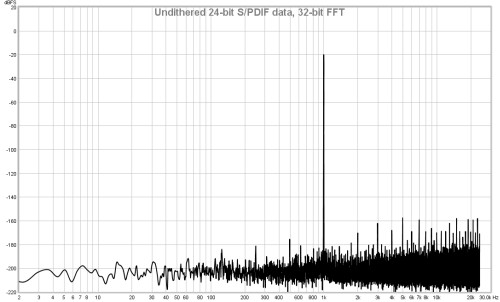
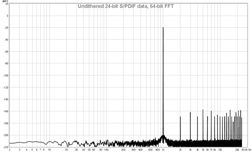
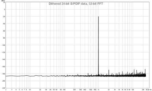
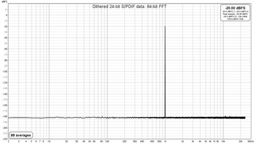
If this option is selected the RTA uses a 64-bit FFT to process the incoming
data instead of 32-bit. This is useful when analysing purely digital 24-bit data paths
to view behaviour below -160 dBFS. It has no visible effect when analysing signals
that have an analog connection at any point along the data path or when dealing with
16-bit data, as in those cases noise and quantisation effects far exceed any numerical
limitations of 32-bit processing. Here are some examples showing the difference the
64-bit FFT makes when analysing undithered and dithered 24-bit data over an S/PDIF
loopback connection from REW's signal generator producing a 1 kHz sine wave at -20 dBFS.
The vertical divisions are at 20 dB intervals, the bottom of the plot is at -220 dBFS.
If this option is selected, the generator is playing a tone burst and the graph is in spectrum mode the peak SPL in the input data will be shown on the plot. This is similar to the CEA-2010 peak SPL but without 1/3 octave filtering around the fundamental frequency.
The Trace options button brings up a dialog that allows the colour and line type of the graph traces to be changed. If a change is made to a measurement trace it will be used for all measurements shown on this graph, overriding the measurement colour. Traces can also be hidden, which will remove them from the graph and from the graph legend.
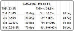
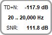
When the Distortion Panel button (keyboard shortcut Alt+D) is selected the analyser calculates and displays harmonic or intermodulation distortion figures for the input, including THD, N+D (A-weighted noise plus distortion), N (noise and non-harmonic distortion), THD+N, SNR (where N excludes harmonic distortion), ENOB, HHD (higher harmonic distortion for harmonics from the 10th up to at most the 50th) and the relative levels of the 2nd to 9th harmonics. N and N+D are displayed in the current Y axis units, harmonic distortion can be displayed as percentages or dB relative to the fundamental depending on the Distortion settings.
If only two inputs are selected for a multi-input RTA measurement distortion figures will be shown individually for each.
Harmonic distortion results are only valid when the system being monitored is driven by a tone or tone burst at a single frequency. If the REW signal generator is playing a sine signal and Fundamental from generator is selected or if the generator is playing a tone burst the generator frequency is used as the fundamental frequency of the input, otherwise the highest peak is used to determine the fundamental. The fundamental and its level are displayed, along with the voltage gain if the signal generator is playing a sine signal. If the Use AES17-2015 standard notch option is selected in the Distortion settings the fundamental figure will be the power within a one octave span around the fundamental frequency. If that option is not selected it will be the power in the main lobe of the fundamental.
When the stimulus is a tone burst the tone burst envelope has a strong spectral spreading effect, which (depending on the envelope shape) means only relatively high levels of distortion can be measured. The distortion calculations use the level from the FFT bin closest to the fundamental and harmonic frequencies. Noise-related results are not calculated as they would not be meaningful.
When calculating the power for the fundamental and harmonics for a continuous tone the energy in the FFT bins within the relevant span of the nominal frequencies appropriate for the RTA window selection is summed and then corrected according to the window's equivalent noise bandwidth. To obtain accurate results the window should have low side lobes. Good choices in order of reducing side lobe level are Dolph-Chebyshev 150 (side lobes 150 dB down), Blackman-Harris 7 (side lobes 180 dB down), Dolph-Chebyshev 200 (side lobes 200 dB down) and Cosine sum 9-235 (side lobes 235 dB down). Hann, Blackman-Harris 4 and Flat-Top are not recommended. If using the REW signal generator the option to lock frequency to the RTA FFT allows a rectangular window to be used.
Dither should be enabled on the generator at the bit width the system is using, check the bottom left corner of the REW main window for the bit width in use. On Windows using Java drivers only 16 bit is supported, for 24-bit use ASIO drivers. On macOS 24-bit is supported, make sure the devices are configured to operate at 24-bit or higher in Audio Midi setup.
The THD figure is based on harmonics up to at most the 50th or the number of harmonics whose levels are displayed and is calculated from the sum of those harmonic powers relative to the power of the fundamental. A separate HHD (higher harmonic distortion) figure is calculated from the sum of harmonic powers for the 10th up to at most the 50th harmonic. The THD figure includes the HHD contribution. Individual harmonic figures are also calculated from their power relative to the power of the fundamental.
The THD+N figure is calculated from the ratio of the input power minus the fundamental power to the total input power (note that it is possible for THD+N to be lower than THD using these definitions). Note that the reciprocal of THD+N is SINAD. The N figure is calculated from THD+N minus THD (including all harmonics in the distortion bandwidth), either as a ratio to the total input power if the Y axis units are dBc or as an absolute figure for other Y axis settings.
The upper limit for data used in distortion calculations is 95% of the Nyquist frequency (i.e. 95% of half the sample rate) or the Distortion Low Pass, if enabled. The lower limit is the first FFT bin (DC is excluded) or the distortion High Pass, if enabled.
The example below shows data for a 1 kHz sine input. The positions of the harmonics
are shown on the spectrum or RTA plot. The Distortion High Pass and Distortion Low
Pass have been set to 20 Hz and 20 kHz respectively, hence results are based on
data from the span 20 Hz to 20 kHz.
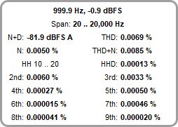
An A-weighted noise plus distortion (N+D) figure is also shown alongside the THD data, in the current Y axis units. Using this figure together with the maximum input level (at distortion of better than -40 dB) allows a dynamic range figure to be generated. For a meaningful N+D result per AES17-2015 the system should be driven with a 997 Hz sine wave at 60 dB below the maximum input level.
Intermodulation distortion results are only valid when the system being monitored is driven using REW's Dual Tone test signal. The signal can be generated live from the generator, or saved to a file and played back on the system being measured. If playing from file the generator must still be showing with the same signal selected so that REW knows what it should calculate.
The generator provides preset signals for SMPTE, DIN, CCIF and AES17-2015 intermodulation measurement signals and a 'Custom' option allowing a user-selected pair of frequencies at a 1:1 or 4:1 amplitude ratio. Signals at 1:1 ratio will begin to clip at -3.0 dBFS (with the View option Full scale sine rms is 0 dBFS selected, 3 dB lower otherwise). Signals at 4:1 ratio will clip at -1.8 dBFS.
Dither should be enabled on the generator at the bit width the system is using, check the bottom left corner of the REW main window for the bit width in use. On Windows using Java drivers only 16 bit is supported, for 24-bit use ASIO drivers. On macOS 24-bit is supported, make sure the devices are configured to operate at 24-bit in Audio Midi setup.
To obtain accurate results the RTA window should have very low side lobes.
Good choices in order of reducing side lobe level are Dolph-Chebyshev 150 (side lobes
150 dB down), Blackman-Harris 7 (side lobes 180 dB down), Dolph-Chebyshev 200 (side lobes
200 dB down) and Cosine sum 9-235 (side lobes 235 dB down). Do not use the Hann,
Blackman-Harris 4 or Flat-Top windows.
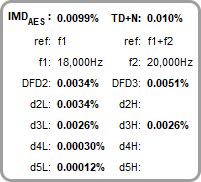
The CCIF figure is calculated from the level at f2 - f1 (also called the 2nd order Difference Frequency Distortion or DFD2). The 3rd order DFD3 figure based on the levels at 2*f1 - f2 (18 kHz) and 2*f2 - f1 (21 kHz) is also shown. The reference level for the DFD figures is the sum of the level at f1 and the level at f2. An IMDpwr figure is also shown, which is the ratio of the rms sums of the IMD components to the rms sum of f1, f2 and the IMD components.
The TDFD IMDTDFD is calculated from the rms sum of 2nd order and 3rd order components, the reference level for the percentage figure is the sum of the levels at f1 and f2. For TDFD Phono and TDFD akl d2L (f2 - f1) and d3L (2*f1 - f2) are used, for TDFD Bass d2H (f2 + f1) and d3H (2*f2 - f1) are used.
The AES17 DFD IMDAES figure is based on the levels at f2 - f1 (2 kHz), 2*f1 - f2 (16 kHz) and 2*f2 - f1 (22 kHz), the reference level for the IMDAES percentage figure is the level at f1 (18 kHz). In all cases levels are measured across a 500 Hz bandwidth centred on the component being measured, per the AES17-2015 specification. DFD2 and DFD3 are also shown.
The AES17 MD IMDAES is calculated from the rms sum of the 2nd order (d2) components, the reference level for the percentage figure is the level at f2. REW displays the overall IMD figure and the combined 2nd order (MD2 = d2L + d2H) and 3rd order (MD3 = d3L + d3H) figures.
For signals other than AES17 MD with an f2/f1 ratio > 7 (including SMPTE and DIN) the IMDDIN figure is calculated from the rms sum of the 2nd order (d2) and 3rd order (d3) components, the reference level for the percentage figure is the level at f2. REW displays the overall IMD figure and the combined 2nd order (MD2 = d2L + d2H) and 3rd order (MD3 = d3L + d3H) figures. Note that historically SMPTE and DIN IMD were measured using an analog amplitude demodulation technique, where the result included noise within the demodulation pass band. With FFT analysis the individual intermodulation components can be measured and used directly, as described above, reducing the contribution of noise. This method may be referred to as Modulation IMD (MOD IMD).
In all cases REW also shows a total distortion + noise percentage, TD+N. This figure is the square root of the ratio of the noise and distortion powers to the power of the tones.
| DFD Components | MD Components | ||
|---|---|---|---|
| Component | Freq | Component | Freq |
| d2L | f2 - f1 | d2L | f2 - f1 |
| d2H | f2 + f1 | d2H | f2 + f1 |
| d3L | 2*f1 - f2 | d3L | f2 - 2*f1 |
| d3H | 2*f2 - f1 | d3H | f2 + 2*f1 |
| d4L | 3*f1 - 2*f2 | d4L | f2 - 3*f1 |
| d4H | 3*f2 - 2*f1 | d4H | f2 + 3*f1 |
| d5L | 4*f1 - 3*f2 | d5L | f2 - 4*f1 |
| d5H | 4*f2 - 3*f1 | d5H | f2 + 4*f1 |
When the system being monitored is driven using REW's Multitone test signal the RTA shows a figure for total distortion + noise, TD+N. This figure is the square root of the ratio of the power of the noise and distortion components to the power of the tones. The signal generator and signal capture should have the same clock source for the most accurate results, both going through the same device or devices with synchronised sample clocks, and a rectangular window should be used. When the Distortion settings option Monitor clock with multitone is selected REW will measure the replay-to-record clock difference while capturing the signal. If a rectangular window is being used the clock difference is shown as a ppm figure below the distortion results, if the result does not settle at 0.0 ppm the clocks are not synchronised and a window other than rectangular must be used, such as Blackman-Harris 7. If a non-rectangular window is used a longer FFT may be required to resolve low frequency tones in the test signal. If the window is not rectangular but the clock rates do match REW will recommend using a rectangular window to get the most accurate results.
A signal-to-noise ratio figure is also displayed if a rectangular window is being
used and the FFT is two or more times
the signal length, in which case the tones will only occupy bins which are multiples
of (FFT length/signal length) and anything in the other bins will be noise. The noise
figure is obtained by rms summing the noise bins and scaling the result to account for
the proportion of excluded bins. SNR is the ratio of the total rms input level to that
unweighted noise level.
If a multitone measurement is saved the Distortion graph will show plots of the fundamental level (based on the levels of the tones), noise floor and TD+N. The noise floor values are only available if a Rectangular window is being used, generator and capture are using the same clock and the FFT is two or more times the signal length.
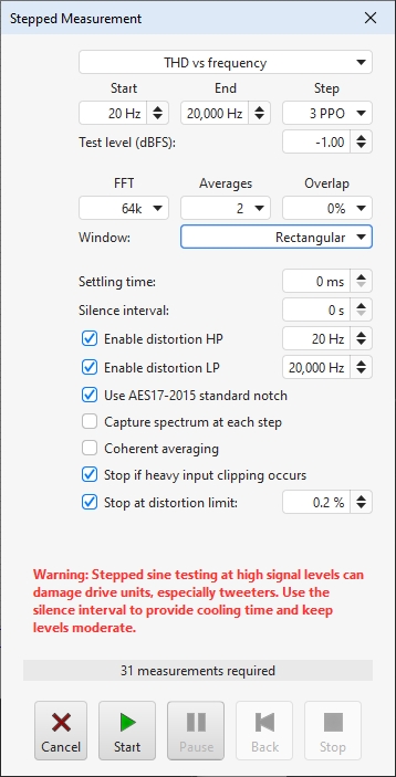
When the Stepped Sine button is pressed a dialog appears to configure and run a stepped sine distortion measurement, stepping in either level or frequency and measuring either harmonic, intermodulation or multitone distortion.
If only two inputs are selected for a multi-input RTA measurement stepped sine measurements can be made for both inputs simultaneously.
REW's signal generator is used to produce the measurement signal. Note that the currently applied signal generator settings are used, so dither will only be applied if selected (it is selected by default and is recommended). The frequency can be stepped in intervals of between 1 and 96 points per octave over the selected span, level can use steps down to 0.1 dBFS. The nominal test frequencies for THD vs frequency will be the preferred values at the chosen measurement PPO that are within the span. To avoid scalloping loss effects the test frequencies use the closest FFT bin frequency, that ensures the peaks of the fundamental and all harmonics are captured in the plots.
At each step all the distortion data is captured, when all points have been captured a new measurement is generated. For THD tests the levels of the fundamental (brown), 2nd harmonic (red), 3rd harmonic (orange) and THD are shown on the RTA graph while the measurement progresses, with solid lines for the first input and dotted lines for the second. IMD tests show the reference level (the level of f1 or f1 plus f2, depending on the stimulus) and the IMD and TD+N levels. Multitone tests show the reference level (the level of the multitone signal) and the TD+N level. If the Stop button is pressed a measurement is generated from the data collected up to that point. Stepped sine measurements typically take many minutes. The Pause button pauses the measurement, turning off the signal generator. Press it again to resume the measurement. The Back button removes the last point measured and re-measures it. Back can be used when the measurement is running or paused. Cancel discards the measurement.
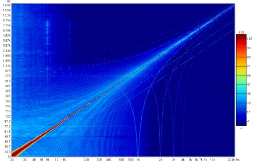
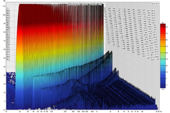
When stepping in frequency a 96 PPO log spaced copy of the spectrum data at each measurement step will be captured if Capture spectrum at each step is selected. That spectrum data can be viewed on the Waterfall or Spectrogram graphs or exported to a text file. Note that exported spectrum data should not be used to try and calculate distortion levels as it does not have sufficient frequency resolution to accurately calculate the energy in each harmonic.
A Settling time in milliseconds can be specified if there are components in the measurement chain which require additional time to settle when the stimulus changes. Each test type has its own settling time setting. A Silence interval in seconds can be specified to allow time for the device being tested to cool between test points.
The Distortion settings for distortion LP, distortion HP, AES17-20155 standard notch and coherent averaging are repeated on this dialog for convenience.
If Stop measurement if heavy input clipping occurs is selected the measurement will be stopped if more than 30% of the samples in an input block are clipped. That corresponds to an input level about 2 dB above the clipping threshold.
If Stop if distortion percentage exceeded is selected the measurement will be stopped if the distortion goes beyond the limit entered. To arm this distortion must first drop below the limit, that allows stepped level measurements to start at low levels, where the distortion figure may be high purely due to noise when the signal level is very low. The distortion check is only carried out on the first input when capturing more than one input. Stepped level measurements have an additional option, If distortion limit hit try smaller step. If that is selected exceeding the distortion limit will pause the measurement, go back to the previous step and continue with a smaller step size until the smallest step (0.1 dB) has been tried. That allows the level at which the distortion limit is reached to be determined more precisely without using a small step for the whole measurement.
When stepping in frequency the minimum start frequency depends on the FFT length and the sample rate - for example, for an 8192 point FFT and 44.1 kHz sample rate the minimum start frequency is approx 60 Hz, for a 32768-point FFT at 44.1 kHz the minimum start is approx 15 Hz. The spreading effect of the RTA window would obscure the 2nd harmonic level at frequencies lower than the minimum and prevent a valid reading of distortion. The measurement frequencies are chosen so that they correspond to bin frequencies for the selected FFT length, this prevents window scalloping loss from affecting the amplitudes of the fundamental or harmonics.
At the beginning of each measurement the noise floor is captured and used to (optionally) mask distortion results that are below the noise floor (see the distortion graph help).
The progress bar shows the approximate time remaining to complete the measurement. Stepped sine measurements are faster when using ASIO drivers as the input and output buffers are smaller than when using Java drivers, hence less time is required for the buffers to flush through when changing frequency or level. The distortion results can be viewed on the Distortion graph. If the Analysis Preference Apply cal files to distortion is selected the results will include corrections for the cal file responses (as is the case for the RTA distortion figures). Applying the cal files provides more accurate results in regions where the fundamental or harmonics are affected by interface roll-offs but boosts the noise floor in those regions. This should be borne in mind when viewing the results. If large cal file corrections are required make sure the Analysis Preference Limit cal data boost to 20 dB is not selected.
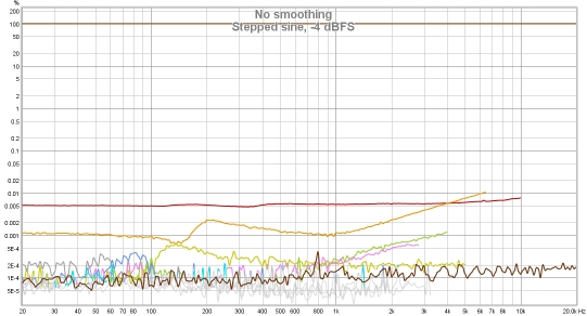
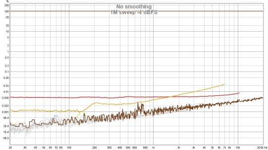
Although much, much slower than a log sweep the stepped sine measurement captures N (noise
and non-harmonic distortion) and THD+N or TD+N (neither is available with a log sweep) and can measure
low distortion levels more accurately than a sweep, particularly at high frequencies and for higher
harmonics. This makes it well suited to measuring the distortion of electronic components. The plots
below show a soundcard loopback measurement at -12 dBFS measured with stepped sine (64k FFT, 24 ppo)
and with 8 repetitions of a 1M log sweep. Note the rise in the levels of harmonics with frequency when
measuring with the sweep. This reflects the rise in the noise floor of the device (as can be viewed with
the RTA in RTA mode), the sweep cannot separate distortion from noise as well as the stepped sine
measurement.