
The graph panel shows plots for the currently selected measurement. The
plots are selected via the buttons at the top of the graph area.
The various graph types are:
SPL and Phase
All SPL
Distortion
Impulse
Filtered IR
Group Delay
RT60
Clarity
Spectral Decay
Waterfall
Spectrogram
Captured
Options that affect the appearance of the traces can be found in the View Preferences.
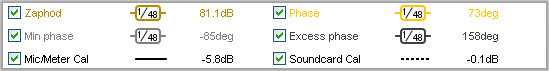
Each trace can be turned on or off via the selection buttons to the left
of the trace name in the legend panel. Trace names are in the same colour
as the trace itself, whilst the line style for the trace is shown between
the label and the trace's value at the current cursor position. If a trace
has smoothing applied the octave fraction is shown (1/12th octave in the
example below). Moving the mouse cursor over a trace name in the legend will
highlight that trace on the graph, fading other traces to help it stand out.
The measurement name can also be shown, this is controlled by the
Show name of highlighted trace preference in the View
Preferences. When a measurement is selected it can be highlighted on overlay
graphs, this is controlled by the Highlight current selection on overlays
preference in the View Preferences. The highlight
state of the current measurement can be toggled using the Ctrl+H shortcut.
Right clicking in the legend area brings up a small menu that allows all traces to be selected, all selections to be cleared or the selections to be toggled. There may be additional options depending on the graph type. A range of traces may be selected by holding the shift key while clicking the selection box for the start of the range then clicking the box for the end of the range.
![]()
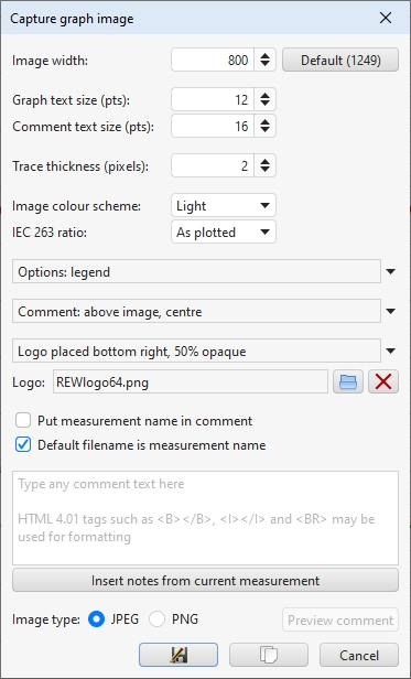
This button at the top left corner of the graph area allows the current
graph view to be captured as an image. It can be activated using the Alt+C shortcut.
A dialog pops up to set the desired width of the image (click Default to
set the image to be the same width as the graph). The thickness of the graph traces
can be selected, the REW default is 2 pixels. There is a selector to choose the colour scheme
for the captured image, which defaults to the current REW coour scheme. If the Include title box is
checked the graph type will be shown at the top of the graph.
IEC 263 ratio is only applicable for graphs that have a horizontal logarithmic frequency axis and a vertical dB axis. It adjusts the vertical size of the captured graph image so that one decade on the frequency axis (e.g. 20 to 200 Hz) has the same length as a 10, 25 or 50 dB span on the dB axis, per the options offered in IEC 263. This ensures a consistent visual appearance of frequency response data and helps avoid graphs that may seem unduly flat or have response slopes that appear shallower or steeper than they are.
There are a set of options for the captured image. If the Include legend box is checked the image includes the graph legend. Include cursor shows the cursor lines and values on the captured image. If Include timestamp is selected the current date and time will be shown at the bottom right corner of the graph. If Monochrome image is selected the traces will be drawn with one of four different line styles instead of in different colours: solid, dotted, dashed or dash-dotted. If Scale overlays is selected and the graph font size chosen for the image is not the same as the current graph font size any overlay boxes on the graph will be scaled correspondingly.
Comments can be placed above, below or on the graph image and aligned to left, right or centre if placed above or below. Comments placed on the graph are centred.
A logo file may be selected and its position and opacity chosen in the options panel below the file chooser.
If Put measurement name in comment is selected the name of the measurement will appear in the comment before any comment text that is entered. If Default filename is measurement name is selected the default name for an image saved to file will be the measurement name. Both options are only available when capturing graphs of single measurements, they are disabled for overlay graph images.
Text typed into the box that shows Type any comment text here will appear on the graph image in the selected Comment position, either above, below or on the graph. Text placed above or below the graph can be styled using HTML 4.01 tags and aligned according to the Comment alignment selection.
The Insert notes from current measurement button inserts the notes from the currently selected measurement in the comments. The Preview comment button allows the formatting to be checked before proceeding. Comment text placed on the graph is centred. The graph will be either saved as JPEG or PNG according to the Image type selected, or copied to the clipboard.
![]()
The Scrollbars button toggles scrollbars for the graph area on/off, hiding
the scrollbars provides more room for the graph. The setting is remembered
for the next startup. If the scrollbars are off, the graph can still be moved
by holding down the right mouse button while in the graph area.
![]()
The Freq Axis button toggles the frequency axis between logarithmic and
linear modes. This function is also available via a command in the
Graph menu and the associated shortcut keys.
![]()
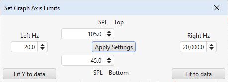
The Graph Limits button allows desired top, left, bottom and right graph limits
to be defined. A dialog pops up in which the values are entered, they are applied
as they are entered or by clicking the Apply Settings button. There are also
buttons to adjust the limits to cover the whole range of the data (Fit to data,
shortcut Ctrl+Alt+F) and to only adjust the Y axis limits to cover the range of the data
leaving the X axis limits unchanged (Fit Y to data, shortcut Ctrl+Alt Y). The
graph limits dialog can also be shown by double-clicking on the graph. The graph limits
can alternatively be adjusted by moving the mouse over the end of a graph axis and using
the mouse wheel or trackpad scroll gesture. Hold the Alt key for fine adjustment when
using the mouse wheel.

The Graph Actions button brings up a menu of actions for the currently selected graph type,
if there are any.
![]()
The Graph Controls button brings up a menu of control options for the currently
selected graph type, if there are any.

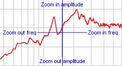
The horizontal axis zoom buttons appear when the mouse pointer is inside the graph
area, they zoom in or out by a factor of approximately 2 centred around the
cursor position. You can also zoom with the keyboard
or by moving the mouse over the graph axis you wish to zoom and using the mouse wheel
or trackpad scroll gesture. Hold the Alt key for fine adjustment when using the mouse wheel.

The vertical axis zoom buttons appear when the mouse pointer is inside
the graph area, they zoom in and out on the Y axis. You can also zoom
with the keyboard or by moving the mouse over
the graph axis you wish to zoom and using the mouse wheel or trackpad scroll
gesture. Hold the Alt key for fine adjustment when using the mouse wheel.
REW provides a variable graphical zoom capability by either pressing and holding the middle mouse button, or pressing the right button then, while the right button is held down, pressing and holding the left button and dragging the pointer.
When variable zoom is active a cross is displayed, split into quadrants allowing horizontal and/or vertical zooming in our out depending on the mouse position. The amount of zoom is governed by how far the mouse pointer is dragged from the start position.
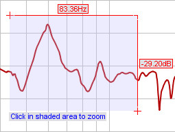
When the Ctrl key is pressed followed by the right mouse button a zoom box can be drawn by dragging the mouse. Note that on a Mac it may be necessary to press both the Ctrl and fn keys, or to hold down Ctrl and drag two fingers on the trackpad. Measurement cursors are shown on the outside of the box, to zoom to the shaded area click within it. If the shaded area is too small to zoom in to a message will indicate which dimension is too small for zooming and what the limit is to allow zoom.
The mousewheel can be used to zoom in and out on the graph. Hold the Alt key for fine adjustment. To zoom in the x axis only hold the shift key or move the moue over the X axis. To disable mousewheel zoom see the View preferences.
To zoom in on the horizontal axis press Shift+x, to zoom out press x. To zoom in on the vertical axis press Shift+y, to zoom out press y. The zoom is centred on the cursor position. You may need to click on the graph first.
To undo the last Variable Zoom or Zoom to Area, press Ctrl+Z or select the Undo Zoom entry in the Graph menu. This will restore the graph axes to the settings they had when the right or middle mouse button was last pressed. This Undo feature can be used even if you have not zoomed, just press the right mouse button when the axis settings are to your preference then you can return to these settings (undoing any subsequent movements or control changes) by pressing Ctrl+Z.
The arrow keys can be used to move the graph cursor in single pixel increments. You may need to click on the graph first. To move the graph instead of the cursor, hold down the Shift key while pressing the arrow keys.